
Binned Likelihood Tutorial
The detection, flux determination and spectral modeling of Fermi LAT sources is accomplished by a maximum likelihood optimization technique, as described in the Cicerone (see also, e.g., Abdo, A. A. et al. 2009, ApJS, 183, 46). To illustrate how to use the likelihood software, this narrative gives a step-by-step description for performing a binned likelihood analysis.
You can download this tutorial as a Jupyter notebook and run it interactively. Please see the instructions for using the notebooks with the Fermitools.
Binned vs Unbinned Likelihood
Binned likelihood analysis is the preferred method for most types of LAT analysis (see Cicerone). However, when analyzing data over short time periods (with few events), it is better to use the unbinned analysis. To perform an unbinned likelihood analysis see the Unbinned Likelihood tutorial. A technical document explaining weighted likelihood is available here.
Additional references:
- SciTools References
- Descriptions of available Spectral and Spatial Models
- Examples of XML Model Definitions for Likelihood:
Prerequisites
You will need an event data file, a spacecraft data file (also referred to as the "pointing and livetime history" file), and the current background models (available for download). You may choose to select your own data files, or to use the files provided within this tutorial. Custom data sets may be retrieved from the Lat Data Server.
Outline
- Make Subselections from the Event Data: Since there is computational overhead for each event associated with each diffuse component, it is useful to filter out any events that are not within the extraction region used for the analysis.
- Make Counts Maps from the Event Files: By making simple FITS images we can inspect our data and pick out obvious sources.
- Download the latest diffuse models: The recommended models for a normal point source analysis are gll_iem_v07.fits (a very large file) and iso_P8R3_SOURCE_V3_v1.txt. All of the background models along with a description of the models are available here.
- Create a Source Model XML File: The source model XML file contains the various sources and their model parameters to be fit using the gtlike tool.
- Create a 3D Counts Cube: The binned counts cube is used to reduce computation requirements in regions with large numbers of events.
- Compute Livetimes: Precomputing the livetime for the dataset speeds up the exposure calculation.
- Compute Exposure Cube: This accounts for exposure as a function of energy, based on the cuts made. The exposure map must be recomputed if any change is made to the data selection or binning.
- Compute Source Maps:Here the exposure calculation is applied to each of the sources described in the model.
- Perform the Likelihood Fit: Fitting the data to the model provides flux, errors, spectral indices, and other information.
- Create a Model Map: This can be compared to the counts map to verify the quality of the fit and to make a residual map.
1. Make subselections from the event data
For this case we will use two years of LAT Pass 8 data. This is a longer data set than is described in the Extract LAT Data tutorial.
NOTE: The ROI used by the binned likelihood analysis is defined by the 3D counts map boundary. The region selection used in the data extraction step, which is conical, must fully contain the 3D counts map spatial boundary, which is square.
Selection of data:
- Search Center (RA, DEC) =(193.98, -5.82)
- Radius = 15 degrees
- Start Time (MET) = 239557417 seconds (2008-08-04 T15:43:37)
- Stop Time (MET) = 302572802 seconds (2010-08-04 T00:00:00)
- Minimum Energy = 100 MeV
- Maximum Energy = 500000 MeV
This two-year dataset generates numerous data files. We provide the user with the original event data files and the accompanying spacecraft file:
- L181126210218F4F0ED2738_PH00.fits (5.0 MB)
- L181126210218F4F0ED2738_PH01.fits (10.5 MB)
- L181126210218F4F0ED2738_PH02.fits (6.5 MB)
- L181126210218F4F0ED2738_PH03.fits (9.2 MB)
- L181126210218F4F0ED2738_PH04.fits (7.4 MB)
- L181126210218F4F0ED2738_PH05.fits (6.2 MB)
- L181126210218F4F0ED2738_PH06.fits (4.5 MB)
- L181126210218F4F0ED2738_SC00.fits (256 MB spacecraft file)
In order to combine the two events files for your analysis, you must first generate a text file listing the events files to be included. (If you do not wish to download all the individual files, you can skip to the next step and retrieve the combined, filtered event file. However, you will need the spacecraft file to complete the analysis, so you should retrieve that now.) To generate the file list, type:
prompt> ls *_PH* > binned_events.txt
When analyzing point sources, it is recommended that you include events with high probability of being photons. To do this, you should use gtselect to cut on the event class, keeping only the SOURCE class events (event class 128, or as recommended in the Cicerone). In addition, since we do not wish to cut on any of the three event types (conversion type, PSF, or EDISP), we will use evtype=3 (which corresponds to standard analysis in Pass 7). Note that "INDEF" is the default for evtype in gtselect.
prompt> gtselect evclass=128 evtype=3
Be aware that evclass and evtype are hidden parameters. So to use them, you must type them on the command line.
The text file you made (binned_events.txt) will be used in place of the input fits filename when running gtselect. The syntax requires that you use an @ before the filename to indicate that this is a text file input rather than a fits file.
We perform a selection to the data we want to analyze. For this example, we consider the source class photons within our 15 degree region of interest (ROI) centered on the blazar 3C 279. For some of the selections that we made with the data server and don't want to modify, we can use "INDEF" to instruct the tool to read those values from the data file header. Here, we are only filtering on event class (not on event type) and applying a zenith cut, so many of the parameters are designated as "INDEF".
We apply the gtselect tool to the data file as follows:
prompt>
gtselect evclass=128 evtype=3

Input FT1 file[] @binned_events.txt

Output FT1 file[] 3C279_binned_filtered.fits

RA for new search center (degrees) (0:360) [] INDEF

Dec for new search center (degrees) (-90:90) [] INDEF

radius of new search region (degrees) (0:180) [] INDEF

start time (MET in s) (0:) [] INDEF

end time (MET in s) (0:) [] INDEF

lower energy limit (MeV) (0:) [] 100

upper energy limit (MeV) (0:) [] 500000

maximum zenith angle value (degrees) (0:180) [] 90

Done.

prompt>
In the last step we also selected the energy range and the maximum zenith angle value (90 degrees) as suggested in Cicerone and recommended by the LAT instrument team. The Earth's limb is a strong source of background gamma rays and we can filter them out with a zenith-angle cut. The use of "zmax" in calculating the exposure allows for a more selective method than just using the ROI cuts in controlling the Earth limb contamination. The filtered data are provided here.
After the data selection is made, we need to select the good time intervals in which the satellite was working in standard data taking mode and the data quality was good. For this task we use gtmktime to select GTIs by filtering on information provided in the spacecraft file. The current gtmktime filter expression recommended by the LAT team in the Cicerone is:
(DATA_QUAL>0)&&(LAT_CONFIG==1)
This excludes time periods when some spacecraft event has affected the quality of the data, ensures the LAT instrument was in normal science data-taking mode.
Here is an example of running gtmktime for our analysis of the region surrounding 3C 279.
prompt>gtmktime

Spacecraft data file[] L181126210218F4F0ED2738_SC00.fits

Filter expression[] (DATA_QUAL>0)&&(LAT_CONFIG==1)

Apply ROI-based zenith angle cut[] no

Event data file[] 3C279_binned_filtered.fits

Output event file name[] 3C279_binned_gti.fits

prompt>
The data file with all the cuts described above is provided in this link. A more detailed discussion of data selection can be found in the Data Preparation analysis thread.
To view the DSS keywords in a given extension of a data file, use the gtvcut tool and review the data cuts on the EVENTS extension. This provides a listing of the keywords reflecting each cut applied to the data file and their values, including the entire list of GTIs. (Use the option "suppress_gtis=no" to view the entire list.)
prompt> gtvcut 3C279_binned_gti.fits

Extension name[EVENTS]

DSTYP1: BIT_MASK(EVENT_CLASS,128,P8R3)

DSUNI1: DIMENSIONLESS

DSVAL1: 1:1


DSTYP2: POS(RA,DEC)

DSUNI2: deg

DSVAL2: CIRCLE(193.98,-5.82,15)


DSTYP3: TIME

DSUNI3: s

DSVAL3: TABLE

DSREF3: :GTI


GTIs: (suppressed)


DSTYP4: BIT_MASK(EVENT_TYPE,3,P8R3)

DSUNI4: DIMENSIONLESS

DSVAL4: 1:1


DSTYP4: ENERGY

DSUNI4: MeV

DSVAL4: 100:500000


DSTYP5: ZENITH_ANGLE

DSUNI5: deg

DSVAL5: 0:90

prompt>
Here you can see the event class and event type, the location and radius of the data selection, as well as the energy range in MeV, the zenith angle cut, and the fact that the time cuts to be used in the exposure calculation are defined by the GTI table.
Various Fermitools will be unable to run if you have multiple copies of a particular DSS keyword. This can happen if the position used in extracting the data from the data server is different than the position used with gtselect. It is wise to review the keywords for duplicates before proceeding. If you do have keyword duplication, it is advisable to regenerate the data file with consistent cuts.
2. Make a counts map from the event data
Next, we create a counts map of the ROI, summed over photon energies, in order to identify candidate sources and to ensure that the field looks sensible as a simple sanity check. For creating the counts map, we will use the gtbin tool with the option "CMAP" (no spacecraft file is necessary for this step). Then we will view the output file, as shown below:
prompt> gtbin

Type of output file (CCUBE|CMAP|LC|PHA1|PHA2|HEALPIX) [PHA2] CMAP

Event data file name[] 3C279_binned_gti.fits

Output file name[] 3C279_binned_cmap.fits

Spacecraft data file name[] NONE

Size of the X axis in pixels[] 150

Size of the Y axis in pixels[] 150

Image scale (in degrees/pixel)[] 0.2

Coordinate system (CEL - celestial, GAL -galactic)[] CEL

First coordinate of image center in degrees (RA or galactic l)[] 193.98

Second coordinate of image center in degrees (DEC or galactic b)[] -5.82

Rotation angle of image axis, in degrees[] 0.0

Projection method Projection method e.g. AIT|ARC|CAR|GLS|MER|NCP|SIN|STG|TAN:[] AIT

gtbin: WARNING: No spacecraft file: EXPOSURE keyword will be set equal to ontime.

prompt>  ds9 3C279_binned_cmap.fits &
We chose an ROI of 15 degrees, corresponding to 30 degrees in diameter. Since we want a pixel size of 0.2 degrees/pixel, then we must select 30/0.2=150 pixels for the size of the x and y axes. The last command launches the visualization tool ds9 and produces a display of the generated counts map.
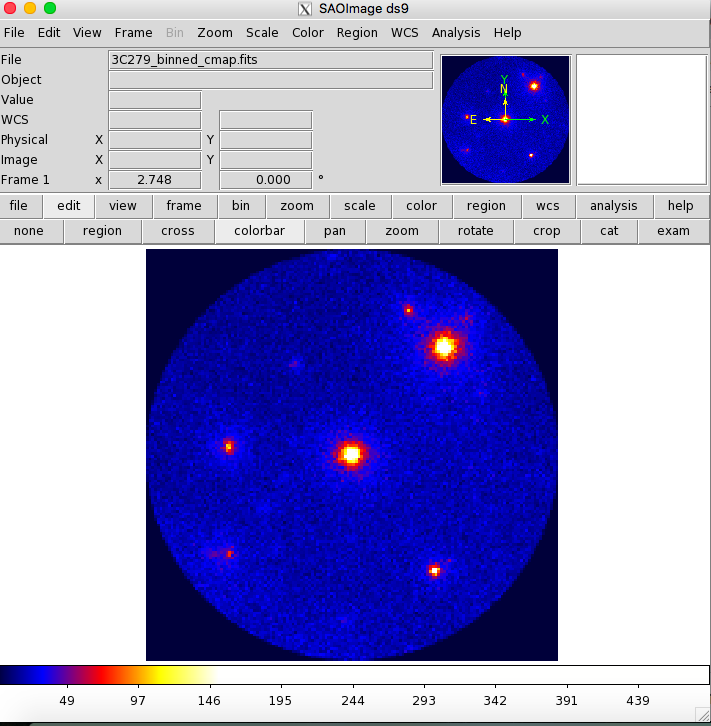
You can see several strong sources and a number of weaker sources in this map. Mousing over the positions of these sources shows that two of them are likely 3C 279 and 3C 273. It is important to inspect your data prior to proceeding to verify that the contents are as you expect. A malformed data query or improper data selection can generate a non-circular region, or a file with zero events. By inspecting your data prior to analysis, you have an opportunity to detect such issues early in the analysis. (A more detailed discussion of data exploration can be found in the Explore LAT Data analysis thread.)
3. Create a 3-D (binned) counts map
Since the counts map shows the expected data, you are ready to prepare your data set for analysis. For binned likelihood analysis, the data input is a three-dimensional counts map with an energy axis, called a counts cube. The gtbin tool performs this task as well, by using the CCUBE option.
 The binning of the counts map determines the binning of the exposure calculation. The likelihood analysis may lose accuracy if the energy bins are not sufficiently narrow to accommodate more rapid variations in the effective area with decreasing energy below a few hundred MeV. For a typical analysis, ten logarithmically spaced bins per decade in energy are recommended. The analysis is less sensitive to the spatial binning and 0.2 deg bins are a reasonable standard.
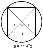
This counts cube is a square binned region that must fit within the circular acceptance cone defined during the data extraction step, and visible in the counts map above. To find the maximum size of the region your data will support, find the side of a square that can be fully inscribed within your circular acceptance region (multiply the radius of the acceptance cone by sqrt(2)). For this example, the maximum length for a side is 21.21 degrees.
To create the counts cube we run gtbin as follows:
prompt> gtbin

Type of output file (CCUBE|CMAP|LC|PHA1|PHA2|HEALPIX) [CMAP] CCUBE

Event data file name[] 3C279_binned_gti.fits

Output file name[] 3C279_binned_ccube.fits

Spacecraft data file name[] NONE

Size of the X axis in pixels[] 100

Size of the Y axis in pixels[] 100

Image scale (in degrees/pixel)[] 0.2

Coordinate system (CEL - celestial, GAL -galactic) (CEL|GAL)[] CEL

First coordinate of image center in degrees (RA or galactic l)[] 193.98

Second coordinate of image center in degrees (DEC or galactic b)[] -5.82

Rotation angle of image axis, in degrees[] 0.0

Projection method Projection method e.g. AIT|ARC|CAR|GLS|MER|NCP|SIN|STG|TAN:[] AIT

Algorithm for defining energy bins (FILE|LIN|LOG)[] LOG

Start value for first energy bin in MeV[] 100

Stop value for last energy bin in MeV[] 500000

Number of logarithmically uniform energy bins[] 37

gtbin: WARNING: No spacecraft file: EXPOSURE keyword will be set equal to ontime.

prompt>
The counts cube generated in this step is provided here. If you open the file with ds9, you see that it is made up of 37 images, one for each logarithmic energy bin. By playing through these images, it is easy to see how the PSF of the LAT changes with energy. You can also see that changing energy cuts could be helpful when trying to optimize the localization or spectral information for specific sources. Be sure to verify that there are no black corners on your counts cube. These corners correspond to regions with no data, and will cause errors in your exposure calculations.
4. Download the latest diffuse model files
When you use the current Galactic diffuse emission model (gll_iem_v07.fits) in a likelihood analysis, you also want to use the corresponding model for the extragalactic isotropic diffuse emission, which includes the residual cosmic-ray background. The recommended isotropic model for point source analysis is iso_P8R3_SOURCE_V3_v1.txt. All the Pass 8 background models have been included in the Fermitools distribution, in the $(FERMI_DIR)/refdata/fermi/galdiffuse/ directory. If you use that path in your model, you should not have to download the diffuse models individually.
NOTE: Keep in mind that the isotropic model needs to agree with both the event class and event type selections you are using in your analysis. The iso_P8R3_SOURCE_V3_v1.txt isotropic spectrum is valid only for the latest response functions and only for data sets with front + back events combined. All of the most up-to-date background models along with a description of the models are available here.
5. Create a source model XML file
The gtlike tool reads the source model from an XML file. The model file contains your best guess at the locations and spectral forms for the sources in your data. A source model can be created using the model editor tool, by using the user contributed package LATSourceModel (see also the user-contributed tools page), or by editing the file directly within a text editor. See Section 4 of the the Unbinned Likelihood tutorial for a brief tutorial on installing this package.
Here we cannot use the same source model that was used to analyze six months of data in the Unbinned Likelihood tutorial, as the 2-year data set contains many more significant sources and will not converge. Instead, we will use the 4FGL-DR4 catalog to define our source model by running make4FGLxml, which comes with the LATSourceModel package. To run the tool, you will need to download the current LAT catalog file and place it in your working directory. Then, use the make4FGLxml tool to create an XML model file:
prompt> make4FGLxml gll_psc_v32.xml --event_file 3C279_binned_gti.fits --output_name 3C279_input_model.xml --free_radius 5.0 --norms_free_only True --sigma_to_free 25 --variable_free True
Note that we are using a high level of significance so that we only fit the brightest sources and we have forced the extended sources to be modeled as point sources.
It is also necessary to specify the entire path to location of the diffuse model on your system. Clearly, the simple 4-source model we used for the 6-month Unbinned Likelihood analysis would have been too simplistic.
This XML file uses the spectral model from the 4FGL-DR4 catalog analysis for each source. (The catalog file is available at the LAT 14-yr Catalog page.) However, that analysis used a subset of the available spectral models. A dedicated analysis of the region may indicate a different spectral model is preferred. For more details on the options available for your XML models, see:
- Descriptions of available Spectral and Spatial Models
- Examples of XML Model Definitions for Likelihood
Finally, the make4FGLxml tool automatically adds 10 degrees to your ROI to account for sources that lie outside your data region, but which may contribute photons to your data. In addition, it gives you the ability to free only some of the spectral parameters for sources within your ROI, and fixes them for the others. With hundreds of sources, there are too many free parameters to gain a good spectral fit. It is advisable to revise these values so that only sources near your source of interest, or very bright source, have all spectral parameters free. Farther away, you can fix the spectral form and free only the normalization parameter (or "prefactor"). If you are working in a crowded region, or have nested sources (e.g. a point source on top of an extended source), you will probably want to fix parameters for some sources even if they lie close to your source of interest.
Only the normalization parameter will be left free (--norms_free_only True) for the remaining sources within the ROI. We have also used the significance parameter (--sigma_to_free 25) of make4FLGxml to free only the brightest sources in our ROI. In addition, we used the variability parameter (--variable_free True) to override that for sources that are significantly variable. We also use a limit of five degrees from the center of the search region (--free_radius 5.0) to reduce the number of sources with free parameters. These changes are necessary: having too many free parameters will not allow the fit to converge (see the section for the fitting step).
The XML file used in this example can be found here. This file was made with an earlier version of the LAT catalog, so it will contain fewer sources and some of those sources will have different spectral shapes/parameter values. These changes may cause the likelihood analysis step to fail to reach convergence. For a discusssion of this issue and some suggestions for how to mitigate it, see the "Run the Likelihood Analysis" section of the Likelihood Analysis with Python thread.
XML for Extended Sources
In some regions, the make4FGLxml script may add one or more extended sources to your XML model. The script will provide the number of extended sources included in the model. In order to use these extended sources, you will need to downloaded the extended source templates from the LAT Catalog page (look for "Extended Source template archive"). Extract the archive in the directory of your choice and note the path to the template files, which have names like "W44.fits" and "VelaX.fits". You will need to provide the path to the template file to the script before you run it.
Here is an example of the proper format for an extended source XML entry for Binned Likelihood analysis:
<source name="SpatialMap_source" type="DiffuseSource">

	<spectrum type="PowerLaw2">

		<parameter free="1" max="1000.0" min="1e-05" name="Integral" scale="1e-06" value="1.0"/>

		<parameter free="1" max="-1.0" min="-5.0" name="Index" scale="1.0" value="-2.0"/>

		<parameter free="0" max="200000.0" min="20.0" name="LowerLimit" scale="1.0" value="20.0"/>

		<parameter free="0" max="200000.0" min="20.0" name="UpperLimit" scale="1.0" value="2e5"/>

	</spectrum>

	<spatialModel W44 file="$(PATH_TO_FILE)/W44.fits" type="SpatialMap" map_based_integral="true">

		<parameter free="0" max="1000.0" min="0.001" name="Normalization" scale= "1.0" value="1.0"/>

	</spatialModel>

</source>
6. Compute livetimes and exposure
To speed up the exposure calculations performed by Likelihood, it is helpful to pre-compute the livetime as a function of sky position and off-axis angle. The gtltcube tool creates a livetime cube, which is a HealPix table, covering the entire sky, of the integrated livetime as a function of inclination with respect to the LAT z-axis.
Here is an example of how to run gtltcube:
prompt> gtltcube zmax=90

Event data file[] 3C279_binned_gti.fits

Spacecraft data file[] L181126210218F4F0ED2738_SC00.fits

Output file[] 3C279_binned_ltcube.fits

Step size in cos(theta) (0.:1.)[] 0.025

Pixel size (degrees)[] 1

Working on file L181126210218F4F0ED2738_SC00.fits

.....................!

prompt>
Note: Values such as "0.1" for "Step size in cos(theta)" are known to give unexpected results. Use "0.09" instead.
The livetime cube generated for this analysis can be found here. For more information about the livetime cubes see the documentation in the Cicerone, and also the explanation in the Unbinned Likelihood tutorial.
7. Compute exposure map
Next you must apply the livetime calculated in the previous step to your region of interest. To do this, we use the gtexpcube2 tool, which is an updated version of the previous gtexpcube. This tool generates a binned exposure map, an accounting of the exposure at each position in the sky, that are a required input to the likelihood process.
NOTE: In the past, running gtsrcmaps calculated the exposure map for you, so most analyses skipped the binned exposure map generation step. With the introduction of gtexpcube2, this is no longer the case. You must explicitly command the creation of the exposure map as a separate analysis step.
In order to create an exposure map that accounts for contributions from all the sources in your analysis region, you must consider not just the sources included in the counts cube. The large PSF of the LAT means that at low energies, sources from well outside your counts cube could affect the sources you are analyzing. To compensate for this, you must create an exposure map that includes sources up to 10 degrees outside your ROI. (The ROI is determined by the radius you downloaded from the data server, here a 15 degree radius.) In addition, you should account for all the exposure that contributes to those additional sources. Since the exposure map uses square pixels, to match the binning in the counts cube, and to ensure we don't have errors, we generate a 300x300 pixel map.
If you provide gtexpcube2 a filename for your counts cube, it will use the information from that file to define the geometry of the exposure map. This is legacy behavior and will not give you the necessary 20° buffer you need to completely account for the exposure of nearby sources. (It will also cause an error in the next step.) Instead, you should specify the appropriate geometry for the exposure map, remembering that the counts cube used 0.2 degree pixel binning. To do that, enter 'none' when asked for a Counts cube.
Note: If you get a "File not found" error in the examples below, just put the IRF name in explicitly. The appropriate IRF for this data set is P8R3_SOURCE_V3.
prompt> gtexpcube2

Livetime cube file[] 3C279_binned_ltcube.fits

Counts map file[] none

Output file name[] 3C279_binned_expcube.fits

Response functions to use[] P8R3_SOURCE_V3

Size of the X axis in pixels[] 300

Size of the Y axis in pixels[] 300

Image scale (in degrees/pixel)[] .2

Coordinate system (CEL - celestial, GAL -galactic) (CEL|GAL) [] CEL

First coordinate of image center in degrees (RA or galactic l)[] 193.98

Second coordinate of image center in degrees (DEC or galactic b)[] -5.82

Rotation angle of image axis, in degrees[] 0

Projection method e.g. AIT|ARC|CAR|GLS|MER|NCP|SIN|STG|TAN[] AIT

Start energy (MeV) of first bin[] 100

Stop energy (MeV) of last bin[] 500000

Number of logarithmically-spaced energy bins[] 37

Computing binned exposure map....................!
The generated exposure map can be found here.
At this point, you may decide it is easier to simply generate exposure maps for the entire sky. You may be right, as it certainly simplifies the step when scripting. However, making an all-sky map increases the processing time for this step, though the increase is modest. To generate an all-sky exposure map (rather than the exposure map we calculated above) you need to specify the proper binning and explicitly give the number of pixels for the entire sky (360°x180°). Here is an example:
prompt> gtexpcube2

Livetime cube file[] 3C279_binned_ltcube.fits

Counts map file[] none

Output file name[] 3C279_binned_allsky_expcube.fits

Response functions to use[] P8R3_SOURCE_V3

Size of the X axis in pixels[] 1800

Size of the Y axis in pixels[] 900

Image scale (in degrees/pixel)[] .2

Coordinate system (CEL - celestial, GAL -galactic) (CEL|GAL) [] CEL

First coordinate of image center in degrees (RA or galactic l)[] 193.98

Second coordinate of image center in degrees (DEC or galactic b)[] -5.82

Rotation angle of image axis, in degrees[] 0

Projection method e.g. AIT|ARC|CAR|GLS|MER|NCP|SIN|STG|TAN[] AIT

Start energy (MeV) of first bin[] 100

Stop energy (MeV) of last bin[] 500000

Number of logarithmically-spaced energy bins[] 37

Computing binned exposure map....................!
The all-sky exposure map can be found here.
Just as in the Unbinned Likelihood analysis, the exposure needs to be recalculated if the ROI, zenith angle, time, event class, or energy selections applied to the data are changed. For the binned analysis, this also includes the spatial and energy binning of the 3D counts map (which affects the exposure map as well).
8. Compute source map
The gtsrcmaps tool creates model counts maps for use with the binned likelihood analysis. To do this, it takes each source spectrum in the XML model, multiplies it by the exposure at the source position, and convolves that exposure with the effective PSF.
This is an example of how to run the tool:
prompt> gtsrcmaps

Exposure hypercube file[] 3C279_binned_ltcube.fits

Counts map file[] 3C279_binned_ccube.fits

Source model file[] 3C279_input_model.xml

Binned exposure map[] 3C279_binned_allsky_expcube.fits

Source maps output file[] 3C279_binned_srcmaps.fits

Response functions[CALDB]


>Much Output Suppressed<


Generating SourceMap for 4FGL J1118.2-0415....................!

Generating SourceMap for 4FGL J1118.6-1235....................!

Generating SourceMap for 4FGL J1119.9-0011....................!

Generating SourceMap for gll_iem_v07....................!

Generating SourceMap for iso_P8R3_SOURCE_V3_v1....................!

prompt>
The output file from gtsrcmaps can be found here.
Because your model map can include sources outside your ROI, you may see a list of warnings at the beginning of the output. These are expected (because you have properly included sources outside your ROI in your XML file) and should cause no problem in your analysis. In addition, if your exposure map is too small for the region, you will see the following warning:
Caught St13runtime_error at the top level:

Request for exposure at a sky position that is outside of the map boundaries.


The contribution of the diffuse source outside of the exposure

and counts map boundaries is being computed to account for PSF

leakage into the analysis region. To handle this, use an all-sky

binned exposure map. Alternatively, to neglect contributions

outside of the counts map region, use the emapbnds=no option when

running gtsrcmaps.
In this situation, you should increase the dimensions of your exposure map, or just move to the all-sky version.
Source map generation for the point sources is fairly quick, and maps for many point sources may take up a lot of disk space. If you are analyzing a single long data set, it may be preferable to pre-compute only the source maps for the diffuse components at this stage. gtlike will compute maps for the point sources on the fly if they appear in the XML definition and a corresponding map is not in the source maps FITS file. To skip generating source maps for point sources, specify "ptsrc=no" on the command line when running gtsrcmaps. However, if you expect to perform multiple fits on the same set of data, precomputing the source maps will probably save you time.
9. Run gtlike
NOTE: Prior to running gtlike for Unbinned Likelihood, it is necessary to calculate the diffuse response for each event (when that response is not precomputed). However, for Binned Likelihood analysis the diffuse response is calculated over the entire bin, so this step is not necessary. In order to use the energy dispersion correction during your analysis, please refer to the dedicated page.
Now we are ready to run the gtlike application. Here, we request that the fitted parameters be saved to an output XML model file for use in later steps.
prompt> gtlike refit=yes plot=yes sfile=3C279_binned_output.xml


Statistic to use (BINNED|UNBINNED)[] BINNED

Counts map file[] 3C279_binned_srcmaps.fits

Binned exposure map[] 3C279_binned_allsky_expcube.fits

Exposure hypercube file[] 3C279_binned_ltcube.fits

Source model file[] 3C279_input_model.xml

Response functions to use[] CALDB

Optimizer (DRMNFB|NEWMINUIT|MINUIT|DRMNGB|LBFGS)[] NEWMINUIT
Most of the entries prompted for are fairly obvious. In addition to the various XML and FITS files, the user is prompted for a choice of IRFs, the type of statistic to use, and the optimizer.
The statistics available are:
- UNBINNED This should be used for short timescale or low source count data. If this option is chosen then parameters for the spacecraft file, event file, and exposure file must be given. See explanation in: Likelihood Tutorial
- BINNED This is a standard binned analysis, described in this tutorial. This analysis is used for long timescale or high-density data (such as in the Galactic plane) which can cause memory errors in the unbinned analysis. If this option is chosen then parameters for the source map file, livetime file, and exposure file must be given.
There are five optimizers from which to choose: DRMNGB, DRMNFB, NEWMINUIT, MINUIT and LBFGS. Generally speaking, the faster way to find the parameter estimates is to use DRMNGB (or DRMNFB) to find initial values and then use MINUIT (or NEWMINUIT) to find more accurate results. If you have trouble achieving convergence at first, you can loosen your tolerance by setting the hidden parameter ftol on the command line. (The default value for ftol is 0.001.)
Analyzing a 2-year dataset will take many hours (in our case more than 2 days with a 32-bit machine with 1 GB of RAM). The required running time is high if your source is in the Galactic plane. Here is some output from our fit, where 4FGL J1229.0+0202 and 4FGL J1256.1-0547 corresponds to 3C 273 and 3C 279, respectively:
This is gtlike version


...


Photon fluxes are computed for the energy range 100 to 500000 MeV


4FGL J1229.0+0202:

norm: 4.24961 +/- 0.0168907

alpha: 2.58904 +/- 0.0049473

beta: 0.91588 +/- 0.0356777

Eb: 3.55582

TS value: 31649.4

Flux: 6.65439e-07 +/- 3.60997e-09 photons/cm^2/s


4FGL J1256.1-0547:

Prefactor: 2.12979 +/- 0.00931209

IndexS: 2.34168 +/- 0.00326686

Scale: 1.00464

ExpfactorS: 1.13801 +/- 0.0421069

Index2: 0.4264 +/- 0.0473207

TS value: 28689.6

Flux: 4.97029e-07 +/- 3.76658e-09 photons/cm^2/s


...


gll_iem_v07:

Prefactor: 0.848666 +/- 0.00209618

Index: 0

Scale: 100

Flux: 0.000442097 +/- 1.0918e-06 photons/cm^2/s


iso_P8R3_SOURCE_V3_v1:

Normalization: 1.28172 +/- 0.00374132

Flux: 0.000157477 +/- 4.59591e-07 photons/cm^2/s


WARNING: Fit may be bad in range [100, 199.488] (MeV)

WARNING: Fit may be bad in range [251.124, 316.126] (MeV)

WARNING: Fit may be bad in range [1583.67, 1993.6] (MeV)

WARNING: Fit may be bad in range [2509.63, 3976.99] (MeV)

WARNING: Fit may be bad in range [6302.3, 7933.61] (MeV)

WARNING: Fit may be bad in range [39744.4, 50032.1] (MeV)


Total number of observed counts: 207751

Total number of model events: 207363


-log(Likelihood): 73164.17543


Writing fitted model to 3C279_binned_output.xml
Since we selected 'plot=yes' in the command line, a plot of the fitted data appears. (Note: Certain configurations are not producing a plot after gtlike. The FSSC is working on this issue at the moment. Please click here to generate a plot within python.)
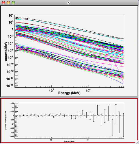
In the first plot the counts/MeV vs MeV are plotted. The points are the data, and the lines are the models. Error bars on the points represent sqrt(Nobs) in that band, where Nobs is the observed number of counts. The black line is the sum of the models for all sources. The colored lines follow the sources as follows:
- Black - summed model
- Red - first source (see below)
- Green - second source
- Blue - third source
- Magenta - fourth source
- Cyan - the fifth source
If you have more sources the colors are reused in the same order. In our case we have, in order of decreasing value on the y-axis: summed model (black), the extragalactic background (black), the galactic background (cyan), 3C 273 (red), and 3C 279 (black).
The second plot gives the residuals between your model and the data. Error bars here represent (sqrt(Nopbs))/Npred, where Npred is the predicted number of counts in each band based on the fitted model.
To assess the quality of the fit, look first for the words at the top of the output "<Optimizer> did successfully converge." Successful convergence is a minimum requirement for a good fit. Next, look at the energy ranges that are generating warnings of bad fits. If any of these ranges affect your source of interest, you may need to revise the source model and refit. You can also look at the residuals on the plot (bottom panel). If the residuals indicate a poor fit overall (e.g., the points trending all low or all high) you should consider changing your model file, perhaps by using a different source model definition, and refit the data.
If the fits and spectral shapes are good, but could be improved, you may wish to simply update your model file to hold some of the spectral parameters fixed. For example, by fixing the spectral model for 3C 273, you may get a better quality fit for 3C 279. Close the plot and you will be asked if you wish to refit the data.
Refit? [y] n

Elapsed CPU time: 1571.805872

prompt>
Here, hitting 'return' will instruct the application to fit again. We are happy with the result, so we type 'n' and end the fit.
Results
When it completes, gtlike generates a standard output XML file. If you re-run the tool in the same directory, these files will be overwritten by default. Use the clobber=no option on the command line to keep from overwriting the output files.
Unfortunately, the fit details and the value for the -log(likelihood) are not recorded in the automatic output files. You should consider logging the output to a text file for your records by using '> fit_data.txt' (or something similar) with your gtlike command. Be aware, however, that this will make it impossible to request a refit when the likelihood process completes.
prompt> gtlike plot=yes sfile=3C279_output_model.xml | tee fit_data.txt
In this example, we used the 'sfile' parameter to request that the model results be written to an output XML file. This file contains the source model results that were written to results.dat at the completion of the fit.
Note: If you have specified an output XML model file and you wish to modify your model while waiting at the 'Refit? [y]' prompt, you will need to copy the results of the output model file to your input model before making those modifications.
The results of the likelihood analysis have to be scaled by the quantity called "scale" in the XML model in order to obtain the total photon flux (photons cm-2 s-1) of the source. You must refer to the model formula of your source for the interpretation of each parameter. In our example the 'prefactor' of our power law model of the source
4FGL J1201.1-0332 has to be scaled by the factor 'scale'=4.7x10⁻¹⁵. For example the total flux of 4FGL J1201.1-0332 is the integral between 100 MeV and 500000 MeV of:
Prefactor x scale x (E /2436)index=(2.7x10-14) * (E/2436)-2.08
Errors reported with each value in the results.dat file are 1σ estimates (based on inverse-Hessian at the optimum of the log-likelihood surface).
Other Useful Hidden Parameters
If you are scripting and wish to generate multiple output files without overwriting, the 'results' and 'specfile' parameters allow you to specify output filenames for the results.dat and counts_spectra.fits files respectively.
If you do not specify a source model output file with the 'sfile' parameter, then the input model file will be overwritten with the latest fit. This is convenient as it allows the user to edit that file while the application is waiting at the 'Refit? [y]' prompt so that parameters can be adjusted and set free or fixed. This would be similar to the use of the "newpar", "freeze", and "thaw" commands in XSPEC.
10. Create a model map
For comparison to the counts map data, we create a model map of the region based on the fit parameters. This map is essentially an infinite-statistics counts map of the region-of-interest based on our model fit.
The gtmodel application reads in the fitted model, applies the proper scaling to the source maps, and adds them together to get the final map.
prompt>gtmodel

Source maps file [] 3C279_binned_srcmaps.fits

Source model file [] 3C279_binned_output.xml

Output file [] 3C279_model_map.fits

Response functions [] CALDB

Exposure cube [] 3C279_binned_ltcube.fits

Binned exposure map [] 3C279_binned_allsky_expcube.fits

prompt>
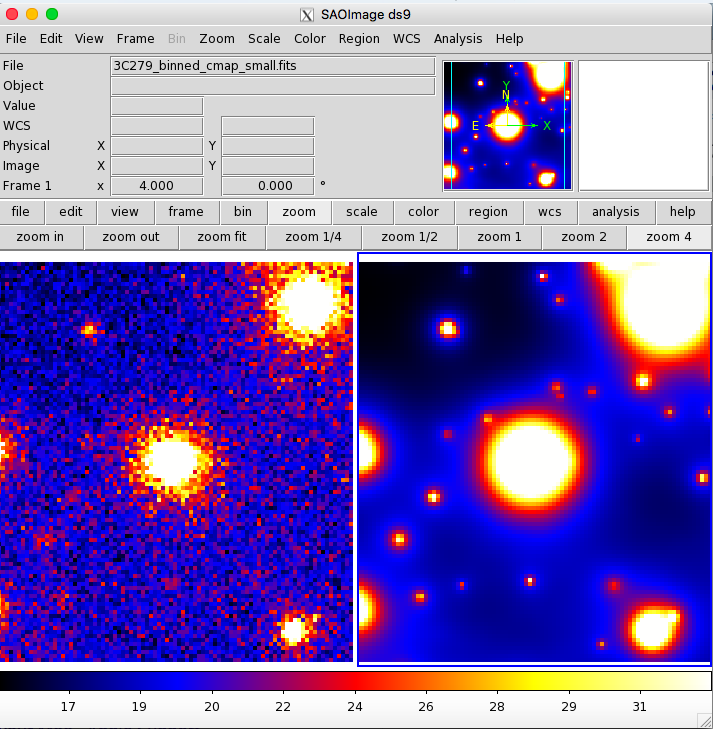
To understand how well the fit matches the data, we want to compare the model map just created with the counts map over the same field of view. First we have to create the new counts map that matches in size the model map (the one generated in encircles the ROI, while the model map is completely inscribed within the ROI): We will use again the gtbin tool with the option "CMAP" as shown below:
prompt> gtbin

Type of output file (CCUBE|CMAP|LC|PHA1|PHA2|HEALPIX) [PHA2] CMAP

Event data file name[] 3C279_binned_gti.fits

Output file name[] 3C279_binned_cmap_small.fits

Spacecraft data file name[] NONE

Size of the X axis in pixels[] 100

Size of the Y axis in pixels[] 100

Image scale (in degrees/pixel)[] 0.2

Coordinate system (CEL - celestial, GAL -galactic)[] CEL

First coordinate of image center in degrees (RA or galactic l)[] 193.98

Second coordinate of image center in degrees (DEC or galactic b)[] -5.82

Rotation angle of image axis, in degrees[] 0.0

Projection method Projection method e.g. AIT|ARC|CAR|GLS|MER|NCP|SIN|STG|TAN:[AIT] STG

gtbin: WARNING: No spacecraft file: EXPOSURE keyword will be set equal to ontime.

prompt>
Here we've plotted the model map next to the the energy-summed counts map for the data.
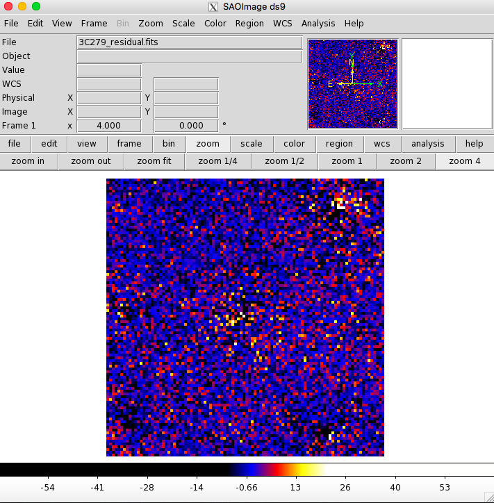
Finally we want to create the residual map by using the FTOOL farith to check if we can improve the model:
prompt> farith

Name of 1st FITS file and [ext#][] 3C279_binned_cmap_small.fits

Name of 2nd FITS file and [ext#][] 3C279_model_map.fits

Name of OUTFIL FITS file[] 3C279_residual.fits

Operation to perform (ADD,SUB,DIV,MUL(or +,-,/,*),MIN,MAX)[] SUB

prompt>
The residual map is shown below. As you can see, the binning we chose probably used pixels that were too large. The primary sources, 3C 273 and 3C 279, have some positive pixels next to some negative ones. This effect could be lessened by either using a smaller pixel size or by offsetting the central position slightly from the position of the blazar (or both). If your residual map contains bright sources, the next step would be to iterate the analysis with the additional sources included in the XML model file.
Last updated by: J. Eggen - 09/13/2023

- Curator: J.D. Myers
- NASA Official: Elizabeth Hays
- Fermi FAQ, Comments, Feedback
- › Privacy Policy and Important Notices
- › Accessibility
- › Contact NASA
- › Page Last Updated: Tue, Nov 28, 2023