
Appendix C. Temporal Analysis with Non-Fermi Analysis Tools
This tutorial illustrates the flow of a basic pulsar analysis, using non-Fermi analysis tools such as XRONOS.
Also see:Steps
- Applying Photon Arrival Time Corrections
- Searching for Pulsations
- Refining and Confirming Ephemeris
- Calculating Pulse Phase for Each Photon
Note
1. Applying Photon Arrival Time Corrections
Sample Files. To try the example in this section yourself, you can download simulated data files below. The simulated data is for demonstration purposes and the simulated pulsar is slightly brighter than the Vela pulsar. For more information, see the parameters used for the simulation.
- fakepulsar_event.fits (372 kB) (Parameters Used)
- simscdata_1week.fits (2.5 MB)
The output file in the example (below) is also available for download for your comparison.
- fakepulsar_event_bary.fits (380 kB)
To use a non-Fermi temporal analysis tool to analyze Fermi data, a Fermi event file may need to be processed for barycentric (or geocentric) corrections, where photon arrival times in a Fermi event file are overwritten by the results of barycentric (or geocentric) corrections, if so expected by the tool. One of the Fermi pulsar tools, gtbary, performs geocentric or barycentric corrections (whichever requested) on all times in a given event file, creates an output file identical to the input file, and overwrites the times in the output file with the corrected times. The times converted by gtbary include all photon arrival times (i.e., the contents of TIME column), good time intervals (in GTI extension), and FITS header keywords storing some kind of time (e.g., TSTART keyword which stores a start time of an observation). Shown below is an example on how to run gtbary to create a converted event file for use with non-Fermi temporal analysis tools. In the following example, gtbary processes the event file named fakepulsar_event.fits using the spacecraft data file named simscdata_1week.fits for a pulsar located at the right ascension of 111.11 and the declination of 22.22, which is the location of the simulated pulsar.
When successful, gtbary creates an output file (fakepulsar_event_bary.fits in the above example) that is ready to be given to a non-Fermi temporal analysis tool that is designed to analyze an event list in the HEASARC standard temporal file format.
Note that, however, once an event file is processed by gtbary, the file needs to be used carefully in your analysis. Not all analysis tools expect an input event file to have been processed by gtbary. Some tools may produce an incorrect result without a warning or an error, if an input event file is already applied barycentric corrections. See the note on Fermi event data processed by gtbary for more details.
2. Searching for Pulsations
Sample Files. To try the example in this section yourself, you can download simulated data files below. The simulated data is for demonstration purposes and the simulated pulsar is slightly brighter than the Vela pulsar. For more information, see the parameters used for the simulation.
- fakepulsar_event_bary.fits (380 kB)
- xronwin.wi (8 kB)
- XRONOS help files: powspec
- XRONOS examples: powspec
- Pulsation Search Tutorial
- SciTools References: gtpspec
If a gamma-ray source of interest has not been recognized as a pulsar (i.e., pulsations have never been detected from the source), or a spin ephemeris for your pulsar is unknown, you may search for pulsations by analyzing Fermi data. In the following example, XRONOS tool powspec reads the event file that is processed by gtbary in the previous section (fakepulsar_event_bary.fits), and computes the Fourier power spectrum of the event data. For more information about XRONOS tool powspec, see XRONOS help file and XRONOS example for powspec.
The computed Fourier power spectrum will be in the output FITS file (powspec_example_1.fits). You can browse it and plot the contents with various FTOOLS such as fv, fdump, and fplot. In the above example, you will find a peak at approximately 12.3449 Hz.
3. Refining and Confirming Ephemeris
Sample Files. To try the example in this section yourself, you can download simulated data files below. The simulated data is for demonstration purposes and the simulated pulsar is slightly brighter than the Vela pulsar. For more information, see the parameters used for the simulation.
- fakepulsar_event_bary.fits (380 kB)
- xronwin.wi (8 kB)
- XRONOS help files: efsearch
- XRONOS examples: efsearch
- Period Search Tutorial
- SciTools References: gtpsearch
Once a spin ephemeris is obtained for your pulsar, either determined by the previous step or simply taken from the literature, you may confirm or refine it by applying statistical tests for periodicity at pulse frequencies near the obtained frequency. In the following example, XRONOS tool efsearch performs the chi-squared test over a range of pulse frequencies on the series of event times processed by gtbary in the previous section (fakepulsar_event_bary.fits). For more information about XRONOS tool efsearch, see XRONOS help file and XRONOS example for efsearch.
The computed chi-squared statistics will be in the output FITS file (efsearch_example_1.fits). You can browse it and plot the contents with various FTOOLS such as fv, fdump, and fplot. In the above example, you will find a peak at approximately 0.081004455 s.
4. Calculating Pulse Phase for Each Photon
Sample Files. To try the example in this section yourself, you can download simulated data files below. The simulated data is for demonstration purposes and the simulated pulsar is slightly brighter than the Vela pulsar. For more information, see the parameters used for the simulation.
- fakepulsar_event.fits (372 kB)
- simscdata_1week.fits (2.5 MB)
- fakepulsar_ephemeris.par (8 kB)
- TEMPO2 plug-in for phase-folding of Fermi photons
- Pulse Phase Calculation Tutorial
- SciTools References: gtpphase
With a spin ephemeris of your pulsar either determined by your analysis or taken from the literature, you can compute a pulse phase for each photon in your Fermi data. Pulse phase values can be used to create a folded light curve to investigate a pulse profile, for example. In the following example, the radio pulsar timing package TEMPO2 with the Fermi plug-in calculates a pulse phase for each photon in a Fermi event data file (fakepulsar_event.fits) based on a spin ephemeris in a text file named fakepulsar_ephemeris.par, using spacecraft positions stored in a Fermi spacecraft file named simscdata_1week.fits, and modifies the event file in place by writing the pulse phase value back to the file. Note that the input file given below is the one not processed by gtbary. That is because TEMPO2 with the Fermi plug-in performs photon arrival time corrections on the fly. As shown below, TEMPO2 with the Fermi plug-in pops up a window showing the results of computations, unless the input file has a very large number of events.
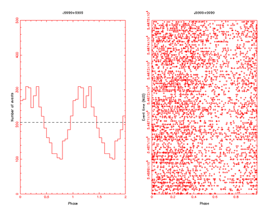
The computed pulse phase values can browsed and plotted with various FTOOLS such as fv, fdump, and fplot. In the above example, a folded light curve shows a sinusoidal pulse profile.
Handle with Care: Fermi Event File Processed by gtbary
In high precision temporal analysis, photon arrival times are converted into times at which the photons would have arrived if the instrument were at a different location. When a source of interest is in a binary system, the converted times are further converted into times at which the photons would have arrived if the photons were emitted at the center of gravity of the binary system. The following table summarizes photon arrival times that are frequently used in pulsar analysis. It also shows the time system normally used for each of these arrival times.
| Time | Photon Emitted at | Photon Arrived at | Time System |
|---|---|---|---|
| Mission Elapsed Time | Photon source (pulsar) | Spacecraft | Mission dependent |
| Geocentric Time | Photon source (pulsar) | Geocenter (Earth's center of gravity) | TT (Terrestrial Time) |
| Barycentric Time | Photon source (pulsar) | Solar system barycenter (Solar system's center of gravity) | TDB (Barycentric Dynamical Time) |
| Binary-demodulated Barycentric Time | Binary system's center of gravity | Solar system barycenter (Solar system's center of gravity) | TDB (Barycentric Dynamical Time) |
By default, the Fermi pulsar analysis tools automatically perform those photon arrival time corrections on the fly, based on the information available (such as solar system ephemerides and binary orbital parameters). This is to preserve original photon arrival times in event files (stored in TIME column), such that other Fermi or non-Fermi analysis tools can use the original times, for example, in order to correctly refer an instrument response for a particular photon without an extra task in an instrument response computations.
Some of the existing temporal analysis tools, however, expect the converted photon arrival times to be written back to the event file, overwriting the original photon arrival times. In fact, this is a commonly-employed convention in various high-energy astrophysics missions, as HEASARC of NASA/GSFC defines and recommends an event file format for temporal analysis in which original photon arrival times are overwritten when geocentric or barycentric corrections are applied. As a result, if a Fermi event file is given to a non-Fermi temporal analysis tool, the tool may not run at all. Even worse the tool may appear to run properly, but only to produce a result that is scientifically incorrect.
Once an event file has been processed by gtbary, the file should not be used as input to any other analysis tools in the Fermi Science Tools package. Because all times written in the file have been replaced by corrected times, if an analysis tool needs to compute a physical quantity at the time of photon arrival, the tool ends up using a corrected time instead of the actual arrival time. This results in quantities such as the spacecraft pointing to be incorrect for the given photon. To prevent this, gtbary marks the file as "already processed for photon arrival time corrections" by changing a set of FITS header keywords (TIMEREF and TIMESYS). Some analysis tools in the Science Tools package recognize it, and refuse to run (i.e., terminate without processing given data and produce an error message). But some other tools do not check those header keywords and assume times recorded in an event file are the original photon arrival times.
A typical case appears in a tempo-spectral analysis, such as a phase-resolved spectral analysis. If one desires to investigate pulse-phase dependency of spectral index, for instance, then a natural approach is to assign pulse phase to each photon, sub-select photons by pulse phase, and perform a spectral fit to an energy spectrum for each pulse phase range. If pulse phase assignment is done with a non-Fermi tool that requires barycentric times in an event file, one can run gtbary before the phase assignment tool. But, if the barycentered (or geocentered) event file is given to the spectral analysis tools in the Science Tools package after pulse phase assignment, instrument response will not be correctly computed because 1) instrument response varies with time as the spacecraft location and attitude changes in time, 2) photon arrival times in the event file have been shifted by barycentric corrections (see the Arrival Time Correction Tutorial for more information about photon arrival time corrections), and 3) the spectral analysis tools do not check if photon arrival time corrections have been applied and use the corrected times as the original photon arrival times.
Last updated by: Masaharu Hirayama 08/24/2009

- Curator: J.D. Myers
- NASA Official: Elizabeth Hays
- Fermi FAQ, Comments, Feedback
- › Privacy Policy and Important Notices
- › Accessibility
- › Contact NASA
- › Page Last Updated: Thu, Sep 26, 2019