

Binned Likelihood Tutorial
The detection, flux determination and spectral modeling of Fermi LAT soures is accomplished by a maximum likelihood optimization techique, as described in the Cicerone (see also e.g. Abdo, A. A. et al. 2009, ApJS, 183, 46). This narrative gives a step-by-step description for performing a binned likelihood analysis.
Binned vs Unbinned Likelihood
Unbinned likelihood analysis is the preferred method for spectral fitting of the LAT data (see Cicerone). However, a binnedanalysis is provided for cases where the unbinned analysis cannot be used. For example, the memory required for the likelihood calculation scales with number of photons and number of sources. This memory usage becomes excessive for long observations of complex regions, necessitating the use of binned analysis. To perform an unbinned likelihood analysis see the Likelihood Tutorial.
Additional references:
- SciTools References
- Descriptions of available Spectral and Spatial Models
- Examples of XML Model Definitions for Likelihood:
Prerequisites
You will need an event data file, a spacecraft data file (also referred to as the "pointing and livetime history" file), and the current isotropic emission model (available for download). You may choose to select your own data files, or to use the files provided within this tutorial. Custom data sets may be retrieved from the Lat Data Server.
Steps
- Make Subselections from the Event Data
Since there is computational overhead for each event associated with each diffuse component, it is useful to filter out any events that are not within the extraction region used for the analysis.
- Make Counts Maps from the Event Files
These simple FITS images let us inspect our data and help to pick out obvious candidate sources.
- Download the latest model for the isotropic background
The latest model is isotropic_iem_v02.txt. All of the background models along with a description of the models are available here.
- Create a Source Model XML File
The source model XML file contains the various sources and their model parameters to be fit using the gtlike tool.
- Create a 3D (Binned) Counts Map
The binned counts map is used to reduce computation requirements in regions with large numbers of vents.
- Compute LivetimesPrecomputing the livetime for the dataset speeds up the exposure calculation.
- Compute Exposure and Source Maps
These are used to correct for exposure, based on the cuts made. The exposure map must be recomputed if any change is made to the data selection or binning.
- Run gtlike
Fitting the data to the model can give flux, errors, spectral index, and more.
- Create a Model Map
These can be compared to the counts map to verify the quality of the fit.
1. Make Subselections from the Event Data
For this case the original extraction of data from the first six months of the mission was done as described in the Extract LAT Data tutorial.
NOTE: The ROI used by the binned likelihood analysis isdefined by the 3D counts map boundary. Region selection used in thedata extraction step, which is conical, must fully contain the 3D counts map spatial boundary, which is square. For this reason, binned likelihood we will need a larger data selection than is used for unbinned.
Selection of data:
- Search Center (RA, DEC) =(193.98, -5.82)
- Radius = 40 degrees
- Start Time (MET) = 239557417 seconds (2008-08-04 T15:43:37)
- Stop Time (MET) = 255398400 seconds (2008-02-04 T00:00:00)
- Minimum Energy = 100 MeV
- Maximum Energy = 100000 MeV
We provide the user with the original event data files (file1 and file2) as well as with the spacecraft data file that we have renamed to 'binned_spacecraft.fits'. In order to combine the two events files for your analysis, you must first generate a text file listing the events files to be included.
prompt> ls *_PH* > binned_events.txt
This text file (binned_events.txt) will be used in place of the input fits filename when running gtselect. The syntax requires that you use an @ before the filename to indicate that this is a text file input rather than a fits file.
When analyzing a point source, it is recommended that you include events with high probability of being photons. To do this, you should use gtselect to cut on the event class, keeping only event classes 3 and 4 (or as recommended in the Cicerone):
prompt> gtselect evclsmin=3 evclsmax=4
Be aware that evclsmin and evclsmax are hidden parameters. So to use them for a cut, you must type them in the command line.
We perform a selection to the data we want to analyze. For this example, we consider the diffuse class photons within a 40 degree region of interest (ROI) centered on the blazar 3C 279. We apply the gtselect tool to the data file asfollows:
prompt> gtselect evclsmin=3 evclsmax=4

Input FT1 file[] @binned_events.txt

Output FT1 file[] 3C279_binnedevents_filtered.fits

RA for new search center (degrees) (0:360) [] 193.98

Dec for new search center (degrees) (-90:90) [] -5.82

radius of new search region (degrees) (0:180) [] 40

start time (MET in s) (0:) [] 239557417

end time (MET in s) (0:) [] 255398400

lower energy limit (MeV) (0:) [] 100

upper energy limit (MeV) (0:) [] 100000

maximum zenith angle value (degrees) (0:180) [] 105

Done.

prompt>
In the last step we also selected the energy range and the maximum zenith angle value (105 degrees) as suggested in the Cicerone. The Earth limb is a stong source of background gamma rays. We get rid of them with a zenith angle cut. The value of 105 degrees is theone most commonly used. The filtered data is provided here.
After the data selection is made one must correctly calculate the exposure. There are several options for calculating livetime depending on your observation type and science goals. For a detailed discussion of these options, see Likelihood Livetime and Exposure in the Cicerone. To deal with the cut on zenith-angle in this analysis, we use the gtmktime tool to exclude the time intervals where the zenith cut intersects the ROI from the list of good time intervals (GTIs). This is especially needed if you are studying a narrow ROI (with a radius of less than 20 degrees), as your source of interest is likely to come quite close to the Earth's limb. To make this correction you have to run gtmktime and answer "yes" at:
Apply ROI-based zenith angle cut [] yes
gtmktime also provides an opportunity to select GTIs by filtering on
information provided in the spacecraft file. The current gtmktime filter expression recommended by the LAT team is:
DATA_QUAL==1 && LAT_CONFIG==1 && ABS(ROCK_ANGLE)<52.
This excludes time periods when some spacecraft event has affected the quality of the data, ensures the LAT instrument was in normal science data-taking mode, and requires that the spacecraft be within the range of rocking angles used during nominal sky-survey observations.
Here is an example of running gtmktime for our analysis of the region surrounding 3C 279.
prompt> gtmktime

Spacecraft data file[] binned_spacecraft.fits

Filter expression[] (DATA_QUAL==1 && LAT_CONFIG==1 && ABS(ROCK_ANGLE)<52)

Apply ROI-based zenith angle cut[] yes

Event data file[] 3C279_binnedevents_filtered.fits

Output event file name[] 3C279_binnedevents_gti.fits
The data with all the cuts described above is provided in this link. A more detailed discussion of data selection can be found in the Data Preparation tutorial.
To view the DSS keywords in a given extension of a data file, use the gtvcut tool and review the data cuts for the EVENTS extension. This provides a listing of the keywords reflecting each cut applied to the data file and their values, including the entire list of GTIs.
prompt> gtvcut suppress_gtis=yes

Input FITS file[] 3C279_binnedevents_gti.fits

Extension name[EVENTS]

DSTYP1: POS(RA,DEC)

DSUNI1: deg

DSVAL1: CIRCLE(193.98,-5.82,40)


DSTYP2: TIME

DSUNI2: s

DSVAL2: TABLE

DSREF2: :GTI


GTIs: (suppressed)


DSTYP3: ENERGY

DSUNI3: MeV

DSVAL3: 100:100000


DSTYP4: EVENT_CLASS

DSUNI4: dimensionless

DSVAL4: 3:3


DSTYP5: ZENITH_ANGLE

DSUNI5: deg

DSVAL5: 0:105


prompt>
Here you can see the RA, Dec and ROI of the data selection, as well as the energy range in MeV, the event class slesction, the zenith angle cut apllied, and the fact that the time cuts to be used in the exposure calculation are definted by the GTI table.
Various science tools will be unable to run if you have multiple copies of a particular DSS keyword. This can happen if the position used in extracting the data from the data server is different than the position used with gtselect. It is wise to review the keywords for duplicates before proceeding. If you do have keyword duplication, it is advisable to regenerate the data file with consistent cuts.
2. Make Counts Maps from the Event Files
Next, we create a counts map of the region-of-interest (ROI), summed over photon energies, in order to identify candidate sources and to ensure that the field looks sensible as a simple sanity check. For creating the counts map, we will use the gtbin tool with the option "CMAP" as shown below:
prompt> gtbin

This is gtbin version ScienceTools-v9r17p0-fssc-20100630

Type of output file (CCUBE|CMAP|LC|PHA1|PHA2) [] CMAP

Event data file name[] 3C279_binnedevents_gti.fits

Output file name[] 3C279_binned_counts_map.fits

Spacecraft data file name[] NONE

Size of the X axis in pixels[] 320

Size of the Y axis in pixels[] 320

Image scale (in degrees/pixel)[] 0.25

Coordinate system (CEL - celestial, GAL -galactic) (CEL|GAL) [CEL]

First coordinate of image center in degrees (RA or galactic l)[] 193.98

Second coordinate of image center in degrees (DEC or galactic b)[] -5.82

Rotation angle of image axis, in degrees[0.]

Projection method e.g. AIT|ARC|CAR|GLS|MER|NCP|SIN|STG|TAN:[AIT]

prompt>  ds9 3C279_binned_counts_map.fits &
The last command launches the visualization tool ds9 and produces this display:
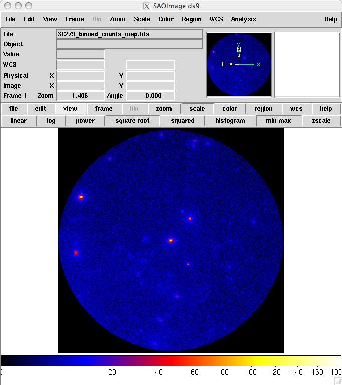
3C279_binned_counts_map.fits
The counts map produced in this step is provided here. From this image you can see that there are no strong sources near the central two sources, 3C 279 and 3C 273.
3. Download the latest background models
When you use the lastest Galactic diffuse emission model, gll_iem_v02.fit, in a likelihood analysis you also want to use the corresponding model for the Extragalactic isotropic diffuse emission, which includes the residual cosmic-ray background. The latest isotropic model is isotropic_iem_v02.txt. For this example, you should save it in the same directory with your data. The isotropic spectrum is valid only for the P6_V3_DIFFUSE response functions and only for data sets with front + back events combined. All of the most up-to-date background models along with a description of the models are available here.
4. Create a Source Model XML File
The gtlike tool reads the source model from an XML file. The source model can be created using the model editor tool or byediting the file directly within a text editor. Review the help information in the model editor to learn how to run this tool.
Given the dearth of bright sources in the extraction region we have selected, our source model file will be fairly simple, comprising only the Galactic and Extragalactic diffuse emission, and point sources to represent the blazars 3C 279 and 3C 273. For this example, we use the diffuse background model as recommended by the LAT Team:
<?xml version="1.0" ?>

<source_library title="source library" xmlns="http://fermi.gsfc.nasa.gov/source_library">

<source name="EG_v02" type="DiffuseSource">

<spectrum file="./isotropic_iem_v02.txt" type="FileFunction">

<parameter free="1" max="1000" min="1e-05" name="Normalization"
scale="1" value="1" />

</spectrum>

<spatialModel type="ConstantValue">

<parameter free="0" max="10.0" min="0.0" name="Value" cale="1.0"
value="1.0"/>

</spatialModel>

</source>


<source name="GAL_v02" type="DiffuseSource">

<!-- diffuse source units are cm^-2 s^-1 MeV^-1 sr^-1 -->

<spectrum type="ConstantValue">

<parameter free="1" max="10.0"
min="0.0" name="Value" scale="1.0" value=
"1.0"/>

</spectrum>

<spatialModel file="$(FERMI_DIR)/refdata/fermi/galdiffuse/gll_iem_v02.fit" type="MapCubeFunction">

<parameter free="0" max="1000.0" min="0.001" name="Normalization" scale=
"1.0" value="1.0"/>

</spatialModel>


</source>

<source name="3C 273" type="PointSource">

<spectrum type="PowerLaw">

<parameter free="1" max="1000.0" min="0.001" name="Prefactor" scale="1e-09" value="10"/>

<parameter free="1" max="-1.0" min="-5.0" name="Index" scale="1.0" value="-2.1"/>

<parameter free="0" max="2000.0" min="30.0" name="Scale" scale="1.0" value="100.0"/>

</spectrum>

<spatialModel type="SkyDirFunction">

<parameter free="0" max="360" min="-360" name="RA" scale="1.0" value="187.25"/>

<parameter free="0" max="90" min="-90" name="DEC" scale="1.0" value="2.17"/>

</spatialModel>

</source>

<source name="3C 279" type="PointSource">

<spectrum type="PowerLaw">

<parameter free="1" max="1000.0" min="0.001" name="Prefactor" scale="1e-09" value="10"/>

<parameter free="1" max="-1.0" min="-5.0" name="Index" scale="1.0" value="-2"/>

<parameter free="0" max="2000.0" min="30.0" name="Scale" scale="1.0" value="100.0"/>

</spectrum>

<spatialModel type="SkyDirFunction">

<parameter free="0" max="360" ="-360" name="RA" scale="1.0" value="193.98"/>

<parameter free="0" max="90" min="-90" name="DEC" scale="1.0" value="-5.82"/>

</spatialModel>
</source>

</source_library>
The XML file used for this example is here. For more details on the available XML models, see:
- Descriptions of available Spectral and Spatial Models
- Examples of XML Model Definitions for Likelihood
5. Create a 3D (Binned) Counts Map
For binned likelihood analysis, a three-dimensional counts map (counts cube) with an energy axis is required. The gtbin aplication performs this tool with the CCUBE option.
The binning of the counts map determines the binning of the exposure calculation. The likelihood analysis may lose accuracy if the energy bins are not sufficiently narrow to accommodate more rapid variations in the effective area with decreasing energy below a few hundred GeV. For a typical analysis, ten logarithmically spaced bins per decade in energy are recommended. The analysis is less sensitive to the spatial binning and 0.2 deg bins are a reasonable standard.
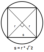
This counts cube is a square binned region that must fit within the circular acceptance cone defined during the data extraction step. This is the reason we expanded the data selection from 20 degrees (for unbinned analysis) to 40 degrees (for binned analysis). To find the maximum size of the region your data will support, find the side of a square that can be fully inscribed within your circular acceptance region (multiply the radius of the acceptance cone by sqrt(2)). For this example, the maxiumum length for a side is 56.56 degrees. This means the entire area covered by the smaller acceptance region (40 degree diameter) used in the unbinned analysis will be included in this analysis as well. For a comparable analysis here, we use the same central coordinate, and a 40x40 degree counts cube.
To create the counts cube we run gtbin as follows:
prompt> gtbin

This is gtbin version ScienceTools-v9r17p0-fssc-20100630

Type of output file (CCUBE|CMAP|LC|PHA1|PHA2) [] CCUBE

Event data file name[] 3C279_binnedevents_gti.fits

Output file name[] 3C279_binned_counts_cube.fits

Spacecraft data file name[NONE]

Size of the X axis in pixels[] 200

Size of the Y axis in pixels[] 200

Image scale (in degrees/pixel)[] 0.2

Coordinate system (CEL - celestial, GAL -galactic) (CEL|GAL) [CEL]

First coordinate of image center in degrees (RA or galactic l)[] 193.98

Second coordinate of image center in degrees (DEC or galactic b)[] -5.82

Rotation angle of image axis, in degrees[0.]

Projection method e.g. AIT|ARC|CAR|GLS|MER|NCP|SIN|STG|TAN:[] AIT

Algorithm for defining energy bins (FILE|LIN|LOG) [LOG]

Start value for first energy bin in MeV[] 100

Stop value for last energy bin in MeV[] 100000

Number of logarithmically uniform energy bins[] 30

prompt>
The counts cube generated in this step is provided in this link. A more detailed discussion of data selection can be found in the Data Preparation tutorial.
6. Compute Livetimes
To speed up the exposure calculations performed by Likelihood, it is helpful to pre-compute the livetime as a function of sky position and off-axis angle. The gtltcube tool creates a livetime cube, which is a HealPix table, covering the full sky, of the integrated livetime as a function of inclination with respect to the LAT z-axis.
Here is an example of how to run gtltcube:
prompt>  gtltcube

Event data file[] 3C279_binnedevents_gti.fits

Spacecraft data file[] binned_spacecraft.fits

Output file[] 3C279_binned_ltcube.fits

Step size in cos(theta) (0.:1.) [0.025]

Pixel size (degrees)[1]

Working on file binnned_spacecraft.fits

.....................!

prompt>
Note: Values such as "0.1" for "Step size in cos(theta)" are known to give unexpected results. Use "0.09" instead.
The livetime cube generated for this analysis can be found here. For more information about the livetime cubes see the documentation in Cicerone, and also the explanation in the Unbinned Likelihood tutorial.
7. Compute Exposure and Source Maps
The gtsrcmaps tool creates a binned exposure map and model counts maps, i.e. multiplied by exposure and convolved with the effective PSF, for use with the binned likelihood analysis. The binning used for the exposure map is taken from the 3D counts map.
This is an example of how to run the tool:
prompt> gtsrcmaps

Exposure hypercube file[] 3C279_ltcube.fits

Counts map file[] 3C279_binned_counts_cube.fits

Source model file[] 3C279_input_model.xml

Binned exposure map[none] 3C279_binned_exposure_map.fits

Source maps output file[] 3C279_srcmaps.fits

Response functions[P6_V3_DIFFUSE]

Generating SourceMap for 3C 273....................!

Generating SourceMap for 3C 279....................!

Generating SourceMap for EG_v02Computing binned exposure map....................!

....................!

Generating SourceMap for GAL_v02....................!

prompt>
While gtsrcmaps is primarily used to generate the binned source maps that are the primary input to the likelihood tool, it also generates the binned exposure map, another required input. If you have run gtsrcmaps previously and there is already an exposure map appropriate for this dataset, you can provide that filename and gtsrcmaps will skip the binned exposure map generation step. Otherwise, gtsrcmaps will compute it using the region and energy bands of the 3D counts map you specify.
Similarly to the unbinned likelihood analysis, the exposure needs to be recalculated if the ROI, zenith angle, time, event class, or energy selections applied to the data are changed. For the binned analysis, this also includes the spatial and energy binning of the 3D counts map.
Since source map generation for the point sources is fairly quick, and maps for many point sources may take up a lot of disk space, it may be preferable to skip pre-computing the source maps for these sources at this stage. gtlike will compute these on the fly if they appear in the XML definition and a corresponding map is not in the source maps FITS file. To skip generating source maps for point sources, specify "ptsrc=no" on the command line when running gtsrcmaps.
8. Run gtlike
NOTE: Prior to running gtlike for Unbinned Likelihood, it is necessary to calculate the diffuse response for each event (when that response is not precomputed). However, for Binned Likelihood analysis the diffuse reponse is calculated over the entire bin, so this step is not necessary.
Now we are ready to run the gtlike application. Here, we request that the fitted parameters be saved to an output XML model file (3C279_output_model.xml) for use in later steps.
prompt> gtlike refit=yes plot=yes sfile=3C279_binned_output_model.xml


Statistic to use (BINNED|UNBINNED)[] BINNED

Counts map file[] 3C279_srcmaps.fits

Binned exposure map[] 3C279_binned_exposure_map.fits

Exposure hypercube file[] 3C279_binned_ltcube.fits

Source model file[] 3C279_input_model.xml

Response functions to use[P6_V3_DIFFUSE]

Optimizer (DRMNFB|NEWMINUIT|MINUIT|DRMNGB|LBFGS)[] NEWMINUIT
Most of the entries prompted for are fairly obvious. In addition to the various XML and FITS files, the user is prompted for a choice of IRFs, the type of statistic to use, the optimizer, and some output file names.
The statistics available are:
- UNBINNED See explanation in: Likelihood Tutorial
- BINNED This is a standard binned analysis, described in this tutorial. If this option is chosen then parameters for the source map file, livetime file, and exposure file must be given.
There are five optimizers from which to choose: DRMNGB, DRMNFB, NEWMINUIT, MINUIT and LBFGS. Generally speaking, the faster way to find the parameters estimation is to use DRMNGB (or DRMNFB) approach to find initial valuend then use MINUIT (or NEWMINUIT) to find more accurate results.
The application proceeds by reading in the spacecraft and event data, and if necessary, computing event responses for each diffuse source.
Here is the output from our fit:
Minuit did successfully converge.

# of function calls: 112

minimum function Value: 270467.253413

minimum edm: 1.6264831e-05


(MORE OUTPUTS HERE...)


Computing TS values for each source (4 total)

....!


3C 273:

Prefactor: 12.5052 +/- 0.521595

Index: -2.75194 +/- 0.0297411

Scale: 100

TS value: 4684.23


3C 279:

Prefactor: 9.93928 +/- 0.354852

Index: -2.32129 +/- 0.0199276

Scale: 100

TS value: 9010.65


EG_v02:

Normalization: 1.12098 +/- 0.0164891


GAL_v02:

Value: 1.3442 +/- 0.0223816

WARNING: Fit may be bad in range [100, 251.189] (MeV)

WARNING: Fit may be bad in range [398.107, 630.957] (MeV)

WARNING: Fit may be bad in range [7943.28, 10000] (MeV)

WARNING: Fit may be bad in range [12589.3, 15848.9] (MeV)

WARNING: Fit may be bad in range [79432.8, 100000] (MeV)


Total number of observed counts: 103025

Total number of model events: 103058


-log(Likelihood): 270467.2591


Writing fitted model to 3C279_binned_output_model.xml
Since we selected 'plot=yes' in the command line, a plot of the fitted data appears.
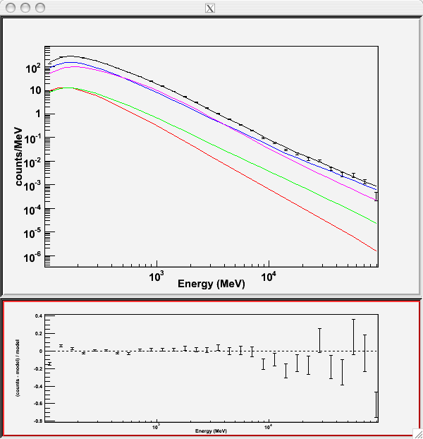
In the first plot the counts/MeV vs MeV are plotted. The points are the data, and the lines are the models. Error bars on the points represent sqrt(Nobs) in that band, where Nobs is the observed number of counts. The black line is the sum of the models for all sources. The colored lines follow the sources as follows:
- Black - summed model
- Red - first source in results.dat file (see below)
- Green - second source
- Blue - third source
- Magenta - fourth source
- Cyan - the fifth source
In our case the 3C273 is the one in red, 3C279 is the one in green, the extragalactic background is blue and the galactic background is magenta. If you have more sources the colors are reused in the same order.
The second plot gives the residuals between your model and the data. Error bars here represent (sqrt(Nopbs))/Npred, where Npred is the predicted number of counts in each band based on the fitted model.
To assess the quality of the fit, look first for the words at the top of the output "<Optimizer> did successfully converge." Successful convergence is a minimum requirement for a good fit. Next, look at the energy ranges that are generating warnings of bad fits. If any of these ranges affect your source of interest, you may need to revise the source model and refit. You can also look at the residuals on the plot (bottom panel). If the residuals indicate a poor fit overall (e.g. the points trending all low or all high) you should consider changing your model file, perhaps by using a different source model definition, and refit the data.
If the fits and spectral shapes are good, but could be improved, you may wish to simply update your model file to hold some of the spectral parameters fixed. For example, by fixing the spectral moel for 3C 273, you may get a better quality fit for 3C 279. Close the plot and you will be asked if you wish to refit the data.
Refit? [y]

n

Elapsed CPU time: 108.232269

prompt>
Here, hitting 'return' will instruct the application to fit again. We are happy with the result, so we type 'n' and end the fit.
Results
When it completes, gtlike generates two standard output files: results.dat with the results of the fit, and counts_spectra.fits with predicted counts for each source for each energy bin. The points in the plot above are the data points from the counts_spectra.fits file, while the colored lines follow the source model information in the results.dat file. If you re-run the tool in the same directory, these files will be overwritten by default. Use the clobber=no option on the command line to keep from overwriting the output files.
Interestingly, the fit details and the value for the -log(likelihood) are not recorded in the automatic output files. You should consider logging the output to a text file for your records by using "> fit_data.txt" (or something similar) with your gtlike command.
prompt> gtlike refit=yes plot=yes sfile=3C279_output_model.xml > fit_data.txt
In this example, we used the 'sfile' parameter to request that the model results be written to an output XML file, 3C279_binned_output_model.xml. This file contains the source model results that were written to results.dat at the completion of the fit.
Note: If you have specified an output XML model file and you wish to modify your model while waiting at the 'Refit? [y]' prompt, you will need to copy the results of the output model file to your input model before making those modifications.
The results of the likelihood analysis have to be scaled by the quantity called "scale" in the XML model in order to obtain the total photon flux (photons cm-2 s-1) of the source. You must refer to the model formula of your source for the interpretation of
each parameter. In our example the 'prefactor' of our power law model of 3C273 has to be scaled by the factor 'scale'=10-9. For example the total flux of 3C273 is the integral between 100 MeV and 100000MeV of:
Prefactor x scale x (E /100)index=(12.5052x10-9) * (E/100)-2.75194
Errors reported with each value in the results.dat file are 1σ estimates (based on inverse-Hessian at the optimum of the log-likelihood surface).
Other Useful Hidden Parameters
If you are scripting and wish to generate multiple output files without overwriting, the 'results' and 'specfile' parameters allow you to specify output filenames for the results.dat and counts_spectra.fits files respectively.
If you wish to include the effects of energy dicpersion in your fit (the significance of this effect depends on each source), you can set the hidden parameter 'edisp=yes' in the command line.
If you do not specify a source model output file with the 'sfile' parameter, then the input model file will be overwritten with the latest fit. This is convenient as it allows the user to edit that file while the application is waiting at the 'Refit? [y]' prompt so that parameters can be adjusted and set free or fixed. This would be similar to the use of the "newpar", "freeze", and "thaw" commands in XSPEC.
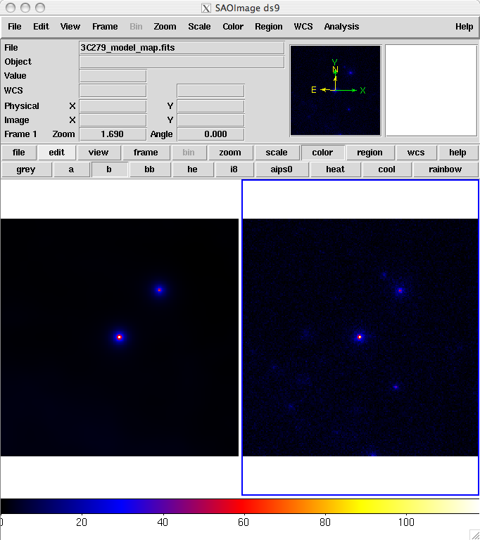
9. Create a Model Map
For comparison to the counts map data, we create a model map of the region based on the fit parameters. This map is essentially an infinite-statistics counts map of the region-of-interest based on our model fit.
The gtmodel application reads in the fitted model, applies the proper scaling to the source maps, and adds them together to get the final map.
prompt>gtmodel

Source maps file [] srcMaps.fits

Source model file []  src_model.xml

Output file [] model_map.fits

Response functions [P6_V3_DIFFUSE]

Exposure cube[] expCube.fits

Binned exposure map[none]  bexposure.fits

prompt>
In order to compare the model results to the data, the two maps must have the same geometry. We generate a counts map for the modeled region using gtbin as before:
prompt> gtbin

This is gtbin version ScienceTools-v9r17p0-fssc-20100630

Type of output file (CCUBE|CMAP|LC|PHA1|PHA2) [] CMAP

Event data file name[] 3C279_binnedevents_gti.fits

Output file name[] 3C279_binned_counts_map_fitted.fits

Spacecraft data file name[] NONE

Size of the X axis in pixels[] 200

Size of the Y axis in pixels[] 200

Image scale (in degrees/pixel)[] 0.2

Coordinate system (CEL - celestial, GAL -galactic) (CEL|GAL) [CEL]

First coordinate of image center in degrees (RA or galactic l)[] 193.98

Second coordinate of image center in degrees (DEC or galactic b)[] -5.82

Rotation angle of image axis, in degrees[0.]

Projection method e.g. AIT|ARC|CAR|GLS|MER|NCP|SIN|STG|TAN:[AIT]
Here we've plotted the model map next to the the energy-summed counts map for the data.
To understand how well the fit matches the data, we subtract the model map from the counts map by using the FTOOL farith.
prompt> farith

Name of 1st FITS file and [ext#][] 3C279_binned_counts_map_fitted.fits

Name of 2nd FITS file and [ext#][] 3C279_model_map.fits

Name of OUTFIL FITS file[] 3C279_residual.fits

Operation to perform (ADD,SUB,DIV,MUL(or +,-,/,*),MIN,MAX)[] SUB

prompt>
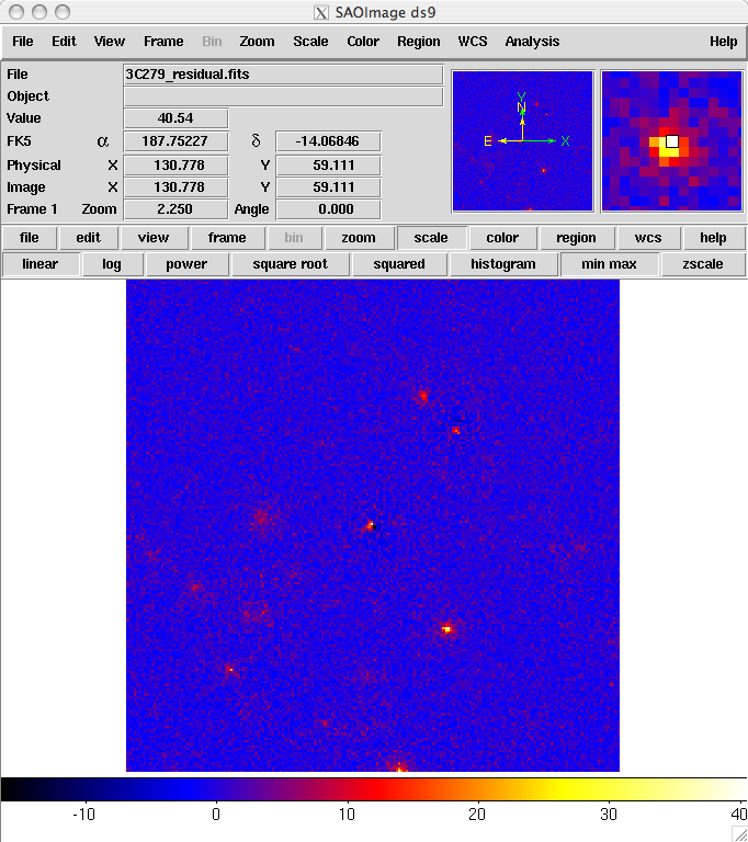
The result is shown below. As you can see, the binning we chose probably used pixels that were too large. The primary source, 3C 279 has a strongly positive pixel next to a strongly negative one. This effect could be lessened by either using a smaller pixel size or by offsetting the central position slightly from the position of the blazar (or both). In addition, the cursor is positioned over a bright source that was not included in our model (this turns out to be a recently identified millisecond pulsar). The next step would be to iterate the analysis with the additional source included in the XML model file.
Last updated by: Elizabeth Ferrara - 01/11/2011