

Likelihood Analysis with Python
The python likelihood tools are a very powerful set of analysis tools that expand upon the command line tools provided with the Fermi Science Tools package. Not only can you perform all of the same likelihood analysis with the python tools that you can with the standard command line tools but you can directly access all of the model parameters, more easily script a standard analysis like light curve generation and there are a few things built into the python tools that are not available from the command line like the calculation of upper limits.
This sample analysis is based on the PG 1553+113 analysis performed by the LAT team and described in Abdo, A. A. et al. 2010, ApJ, 708, 1310. At certain points we will refer to this article as well as the Cicerone. After you complete this tutorial you should be able to reproduce all of the data analysis performed in this publication including generating a spectrum (individual bins and a butterfly plot) and produce a light curve with the python tools. This tutorial uses two user contributed tools (pyLike and make1FGLxml and assumes you have the most recent ScienceTools installed. We will also make significant use of python, so you might want to familiarize yourself with python (there's a beginner's guide at http://wiki.python.org/moin/BeginnersGuide). This tutorial also assumes that you've gone through the non-python based unbinned likelihood thread. This tutorial should take approximately 8 hours to complete (depending on your computer's speed) if you do everything but there are some steps you can skip along the way which shave off about 4 hours of that.
Note: In this tutorial, commands that start with '[user@localhost]$' are to be executed within a shell environment (bash, c-shell etc.) while commands that start with '>>>' are to be executed within an interactive python environment. Commands are in bold and outputs are in normal font. Text in ITALICS within the boxes are comments from the author.
Get the Data
For this thread the original data were extracted from the LAT data server with the following selections (these selections are similar to those in the paper):
- Search Center (RA,Dec) = (238.929,11.1901)
- Radius = 20 degrees
- Start Time (MET) = 239557417 seconds (2008-08-04T15:43:37)
- Stop Time (MET) = 256970880 seconds (2009-02-22T04:48:00)
- Minimum Energy = 100 MeV
- Maximum Energy = 400000 MeV
We've provided direct links to the event files as well as the spacecraft data file if you don't want to take the time to use the download server. For more information on how to download LAT data please see the Extract LAT Data tutorial.
- L110223114519E0D2F37E48_PH00.fits
- L110223114519E0D2F37E48_PH01.fits
- L110223114519E0D2F37E48_SC00.fits
You'll first need to make a file list with the names of your input event files:
[user@localhost]$ ls -1 *PH*.fits > PG1553_events.list
In the following analysis we've assumed that you've named your list of data files PG1553_events.list and the spacecraft file SC.fits.
Perform Event Selections
You could follow the unbinned likelihood tutorial to perform your event selections using gtlike, gtmktime etc. directly from the command line, and then use pylikelihood later. But we're going to go ahead and use python. pyLike (the likelihood module provided by the science tools) provides functions to call these tools from within python. This'll get us used to using python and allow us to build up a script to use later.
So, let's jump into python:
[user@localhost]$ python

Python 2.6.5 (r265:79063, Nov  9 2010, 12:49:33)

[GCC 4.2.1 (Apple Inc. build 5664)] on darwin

Type "help", "copyright", "credits" or "license" for more information.

>>>
Ok, we want to run gtselect inside but we first need to import the gt_apps module to gain access to it.
>>> import gt_apps as my_apps
Now, you can see what objects are part of the gt_apps module by executing
>>> help(my_apps)
Which brings up the help documentation for that module (type 'x' to exit). The python object for gtselect is called filter and we first need to set all of it's options. This is very similar to calling gtselect form the command line and inputting all of the variables interactively. It might not seem that convenient to do it this way but it's really nice once you start building up scripts (see Building a Light Curve) and reading back options and such. For example, towards the end of this thread, we'll want to generate a light curve and we'll have to run the likelihood analysis for each datapoint. It'll be much easier to do all of this within python and change the tmin and tmax in an iterative fashion. Note that these python objects are just wrappers for the standalone tools so if you want any information on their options, see the corresponding documentation for the standalone tool.
>>> my_apps.filter['evclsmin'] = 3

>>> my_apps.filter['evclsmax'] = 4

>>> my_apps.filter['ra'] = 238.929

>>> my_apps.filter['dec'] = 11.1901

>>> my_apps.filter['rad'] = 10

>>> my_apps.filter['emin'] = 200

>>> my_apps.filter['emax'] = 400000

>>> my_apps.filter['zmax'] = 105

>>> my_apps.filter['tmin'] = 239557417

>>> my_apps.filter['tmax'] = 256970880

>>> my_apps.filter['infile'] = '@PG1553_events.list'

>>> my_apps.filter['outfile'] = 'PG1553_filtered.fits'
Once this is done, run gtselect:
>>> my_apps.filter.run()

time -p ~/ScienceTools/i386-apple-darwin10.4.0/bin/gtselect
infile=@PG1553_events.list outfile=PG1553_filtered.fits ra=238.929
dec=11.1901 rad=10.0 tmin=239557417.0 tmax=256970880.0 emin=200.0
emax=400000.0 zmax=105.0 evclsmin=3 evclsmax=4 evclass="INDEF"
convtype=-1 phasemin=0.0 phasemax=1.0 evtable="EVENTS" chatter=2
clobber=yes debug=no gui=no mode="ql"

Done.

real 5.75

user 2.58

sys 1.00
Note that you can see exactly what gtselect will do if you run it by typing:
>>> my_apps.filter.command()

'time -p ~/ScienceTools/i386-apple-darwin10.4.0/bin/gtselect
infile=@PG1553_events.list outfile=PG1553_filtered.fits ra=238.929
dec=11.1901 rad=10.0 tmin=239557417.0 tmax=256970880.0 emin=200.0
emax=400000.0 zmax=105.0 evclsmin=3 evclsmax=4 evclass="INDEF"
convtype=-1 phasemin=0.0 phasemax=1.0 evtable="EVENTS" chatter=2
clobber=yes debug=no gui=no mode="ql"'
You have access to any of the inputs by directly accessing the filter['OPTIONS'] options.
Next, you need to run gtmktime. This is accessed within python via the maketime object:
>>> my_apps.maketime['scfile'] = 'SC.fits'

>>> my_apps.maketime['filter'] = '(DATA_QUAL==1)&&(LAT_CONFIG==1)&&ABS(ROCK_ANGLE)<52'

>>> my_apps.maketime['roicut'] = 'yes'

>>> my_apps.maketime['evfile'] = 'PG1553_filtered.fits'

>>> my_apps.maketime['outfile'] = 'PG1553_filtered_gti.fits'

>>> my_apps.maketime.run()

time -p ~/ScienceTools/i386-apple-darwin10.4.0/bin/gtmktime
scfile=SC.fits sctable="SC_DATA"
filter="(DATA_QUAL==1)&&(LAT_CONFIG==1)&&ABS(ROCK_ANGLE)<52"
roicut=yes evfile=PG1553_filtered.fits evtable="EVENTS"
outfile="PG1553_filtered_gti.fits" apply_filter=yes overwrite=no
header_obstimes=yes tstart=0.0 tstop=0.0 gtifile="default" chatter=2
clobber=yes debug=no gui=no mode="ql"
real 5.57

user 5.05

sys 0.21
We're using the most conservative and most commonly used cuts described in deatil in the Cicerone.
Livetime Cubes and Exposure Maps
At this point, you could make a counts map of the events we just selected using gtbin (it's called evtbin within python) and I won't discourage you but we're going to go ahead and create a livetime cube and exposure map. This might take a few minutes to complete so if you want to create a counts map and have a look at it, get these processes going and open another terminal to work on your counts map (see the likelihood tutorial for an example of running gtbin to produce a counts map).
Livetime Cube
This step will take approximately 30 minutes to complete so if you want to just download the expCube from us you can skip this step.
>>> my_apps.expCube['evfile'] = 'PG1553_filtered_gti.fits'

>>> my_apps.expCube['scfile'] = 'SC.fits'

>>> my_apps.expCube['outfile'] = 'expCube.fits'

>>> my_apps.expCube['dcostheta'] = 0.025

>>> my_apps.expCube['binsz'] = 1

>>> my_apps.expCube.run()

time -p ~/ScienceTools/i386-apple-darwin10.4.0/bin/gtltcube
evfile="PG1553_filtered_gti.fits" evtable="EVENTS" scfile=SC.fits
sctable="SC_DATA" outfile=expCube.fits dcostheta=0.025 binsz=1.0
phibins=0 tmin=0.0 tmax=0.0 file_version="1" zmax=180.0 chatter=2
clobber=yes debug=no gui=no mode="ql"

Working on file SC.fits

.....................!

real 1892.74

user 1848.91

sys 10.58
Exposure Map
>>> my_apps.expMap['evfile'] = 'PG1553_filtered_gti.fits'

>>> my_apps.expMap['scfile'] ='SC.fits'

>>> my_apps.expMap['expcube'] ='expCube.fits'

>>> my_apps.expMap['outfile'] ='expMap.fits'

>>> my_apps.expMap['irfs'] ='P6_V3_DIFFUSE'

>>> my_apps.expMap['srcrad'] =20

>>> my_apps.expMap['nlong'] =120

>>> my_apps.expMap['nlat'] =120

>>> my_apps.expMap['nenergies'] =20

>>> my_apps.expMap.run()

time -p ~/ScienceTools/i386-apple-darwin10.4.0/bin/gtexpmap
evfile=PG1553_filtered_gti.fits evtable="EVENTS" scfile=SC.fits
sctable="SC_DATA" expcube=expCube.fits outfile=expMap.fits
irfs="P6_V3_DIFFUSE" srcrad=20.0 nlong=120 nlat=120 nenergies=20
submap=no nlongmin=0 nlongmax=0 nlatmin=0 nlatmax=0 chatter=2
clobber=yes debug=no gui=no mode="ql"

The exposure maps generated by this tool are meant

to be used for *unbinned* likelihood analysis only.

Do not use them for binned analyses.

Computing the ExposureMap using expCube.fits

....................!

real 53.57

user 51.30

sys 0.72
Generate XML Model File
We need to create an XML file with all of the sources of interest within the Region of Interest (ROI) of PG 1553+113 so we can correctly model the background. For more information on the format of the model file and how to create one, see the likelihood analysis tutorial. We'll use the user contributed tool make1FGLxml.py to create a template based on the LAT 1-year catalog. You'll need to download the FITS version of this file at http://fermi.gsfc.nasa.gov/ssc/data/p6v11/access/lat/1yr_catalog/ and get the make1FGLxml.py tool from the user contributed software page. Also make sure you have the most recent galactic diffuse and isotropic model files which can be found at http://fermi.gsfc.nasa.gov/ssc/data/p6v11/access/lat/BackgroundModels.html.
Now that we have all of the files we need, you can generate your model file in python:
>>> from make1FGLxml import *

This is make1FGLxml version 03.

>>> mymodel = srcList('gll_psc_v02.fit','PG1553_filtered_gti.fits','PG1553_model.xml')

>>> mymodel.makeModel('gll_iem_v02.fit','gal_v02','isotropic_iem_v02.txt','eg_v02')

Creating file and adding sources
For more information on the make1FGLxml module, see the usage notes.
You should now have a file called 'PG1553_model.xml'. Open it up with your favorite text editor and take a look at it. It should look like PG1553_model.xml. There should be three sources (1FGL J1551.7+0851, 1FGL J1553.4+1255 and 1FGL J1555.7+1111) within 3 degrees of the ROI center, four sources (1FGLJ1548.6+1451, 1FGLJ1550.7+0527, 1FGLJ1607.1+1552 and 1FGLJ1609.0+1031) between 3 and 6 degrees and one source between 6 and 9 degrees (1FGLJ1549.3+0235). There are then nine sources beyond 10 degrees. The script designates these as outside of the ROI (which is 10 degrees) and instructs us to leave all of the variables for these sources fixed. We'll agree with this (these sources are outside of our ROI but could still affect our fit since photons from these sources could fall within our ROI). At the bottom of the file, the two diffuse sources are listed (the galactic diffuse and extragalactic isotropic).
Notice that we've deviated a bit from the published paper here. In the paper, the LAT team only included two sources; one from the 0FGL catalog and another, non-catalog source. This is because the 1FGL catalog wasn't released at the time but these 1FGL sources are still in the data we've downloaded and should be modeled. By the way, the 0FGL source ends up being 1FGLJ1553.4+1255 and the 'unknown' source ends up being 1FGLJ1607.1+1552.
Back to looking at our XML model file, notice that all of the sources have been set up with 'PowerLaw' spectral models (see the Cicerone for details on the different spectral models) and the module we ran filled in the values for the spectrum from the 1FGL catalog. How nice! But we're going to re-run the likelihood on these sources anyway just to make sure there isn't anything fishy going on. Also notice that PG 1553+113 is listed in the model file as 1FGL J1555.7+1111 with all of the parameters filled in for us. It's actually offset from the center of our ROI by 0.01 degrees.
So as to make this a little less straight-foward, we going to fit PG 1553+113 with a 'PowerLaw2' spectral model instead of the 'PowerLaw' model it's set as right now. So change the lines associated with 1FGL J1555.7+1111 that look like
<!-- Source is 0.0093446588509 degrees away from ROI center -->
<parameter free="1" max="1e4" min="1e-4" name="Prefactor" scale="1e-12" value="2.41895392605"/>
<parameter free="1" max="5.0" min="0.0" name="Index" scale="-1.0" value="1.66379"/>
<parameter free="0" max="5e5" min="30" name="Scale" scale="1.0" value="2290.660400"/>
</spectrum>
to this
<!-- Source is 0.0093446588509 degrees away from ROI center -->
<parameter free="1" max="1e4" min="1e-4" name="Integral" scale="1e-07" value="0.00586493964505"/>
<parameter free="1" max="5.0" min="0.0" name="Index" scale="-1.0" value="2.21262"/>
<parameter free="0" max="5e5" min="30" name="LowerLimit" scale="1.0" value="2e2"/>
<parameter free="0" max="5e5" min="30" name="UpperLimit" scale="1.0" value="4e5"/>
</spectrum>
Now we're going to do something a little different than the make1FGLxml script gave us.
Run the Likelihood Analysis
It's time to actually run the likelihood analysis now. First, you need to import the pyLikelihood module and then the UnbinnedAnalysis functions (there's also a binned analysis module that you can import to do binned likelihood analysis which behaves almost exactly the same as the unbinned analysis module). As discussed in the likelihood thread it's best to do a two-pass fit here, the first with the DRMNFB optimiser and a looser tolerance and then finally with the NewMinuit optimizer and a tighter tolerance. This allows us to zero in on the best fit parameters and also to obtain the covariance matrix which we'll need in the end (and that the DRMNFB optimizer doesn't provide). For more details on the pyLikelihood module, check out the pyLikelihood Usage Notes.
>>> import pyLikelihood

>>> from UnbinnedAnalysis import *

>>> obs = UnbinnedObs('PG1553_filtered_gti.fits','SC.fits',expMap='expMap.fits',expCube='expCube.fits',irfs='P6_V3_DIFFUSE')

>>> like1 = UnbinnedAnalysis(obs,'PG1553_model.xml',optimizer='DRMNFB')
By now, you'll have two objects, 'obs', an UnbinnedObs object and like1, an UnbinnedAnalysis object. You can view these objects attributes and set them from the command line in various ways. For example:
>>> print obs

Event file(s): PG1553_filtered_gti.fits

Spacecraft file(s): SC.fits

Exposure map: expMap.fits

Exposure cube: expCube.fits

IRFs: P6_V3_DIFFUSE

>>> print like1

Event file(s): PG1553_filtered_gti.fits

Spacecraft file(s): SC.fits

Exposure map: expMap.fits

Exposure cube: expCube.fits

IRFs: P6_V3_DIFFUSE

Source model file: PG1553_model.xml

Optimizer: DRMNFB
or you can get directly at the objects attributes and methods by:
>>> dir(like1)

['NpredValue', 'Ts', 'Ts_old', '_Nobs', '__call__', '__class__', '__delattr__', '__dict__', '__doc__', '__format__', '__getattribute__', '__getitem__', '__hash__',
'__init__', '__module__', '__new__', '__reduce__', '__reduce_ex__', '__repr__', '__setattr__', '__setitem__', '__sizeof__', '__str__', '__subclasshook__', '__weakref__', '_errors',
'_importPlotter', '_inputs', '_isDiffuseOrNearby', '_minosIndexError', '_npredValues', '_plotData', '_plotResiduals',
'_plotSource', '_renorm', '_separation', '_setSourceAttributes', '_srcCnts', '_srcDialog', '_xrange', 'addSource',
'covar_is_current', 'covariance', 'deleteSource', 'disp', 'e_vals', 'energies', 'energyFlux', 'energyFluxError', 'fit', 'flux',
'fluxError', 'freePars', 'freeze', 'getExtraSourceAttributes', 'logLike', 'maxdist', 'minosError', 'model', 'nobs',
'normPar', 'observation', 'oplot', 'optObject', 'optimize', 'optimizer', 'par_index', 'params', 'plot', 'plotSource',
'reset_ebounds', 'resids', 'restoreBestFit', 'saveCurrentFit', 'setFitTolType', 'setFreeFlag', 'setPlotter', 'setSpectrum',
'sourceNames', 'srcModel', 'state', 'syncSrcParams', 'thaw', 'tol', 'tolType', 'total_nobs', 'writeCountsSpectra',
'writeXml']
or get even more details by executing:
>>> help(like1)
There are a lot of attributes and here you start to see the power of using pyLikelihood since you'll be able (once the fit is done) to access any of these attributes directly within python and use them in your own scripts. For example, you can see that the like1 object has a 'tol' attribute which we can read back to see what it is and then set it to what we want it to be.
>>> like1.tol

0.001

>>> like1.tolType

The tolType can be '1' for relative or '0' for absolute.

1

>>> like1.tol = 0.1
Now, we're ready to do the actual fit. This next step will take approximately 5 minutes to complete.
>>> like1.fit(verbosity=0)

271905.89683579269
The number that is printed out here is the -log(Likelihood) of the total fit to the data. You can print the results of the fit by accessing like1.model. You can also access the fit for a particular source by doing the following (the source name must match that in the XML model file).
>>> like1.model['_1FGLJ1555.7+1111']

_1FGLJ1555.7+1111

   Spectrum: PowerLaw2

33      Integral:  5.028e-01  3.033e-02  1.000e-04  1.000e+04 ( 1.000e-07)

34         Index:  1.679e+00  3.341e-02  0.000e+00  5.000e+00 (-1.000e+00)

35    LowerLimit:  2.000e+02  0.000e+00  3.000e+01  5.000e+05 ( 1.000e+00) fixed

36    UpperLimit:  4.000e+05  0.000e+00  3.000e+01  5.000e+05 ( 1.000e+00) fixed
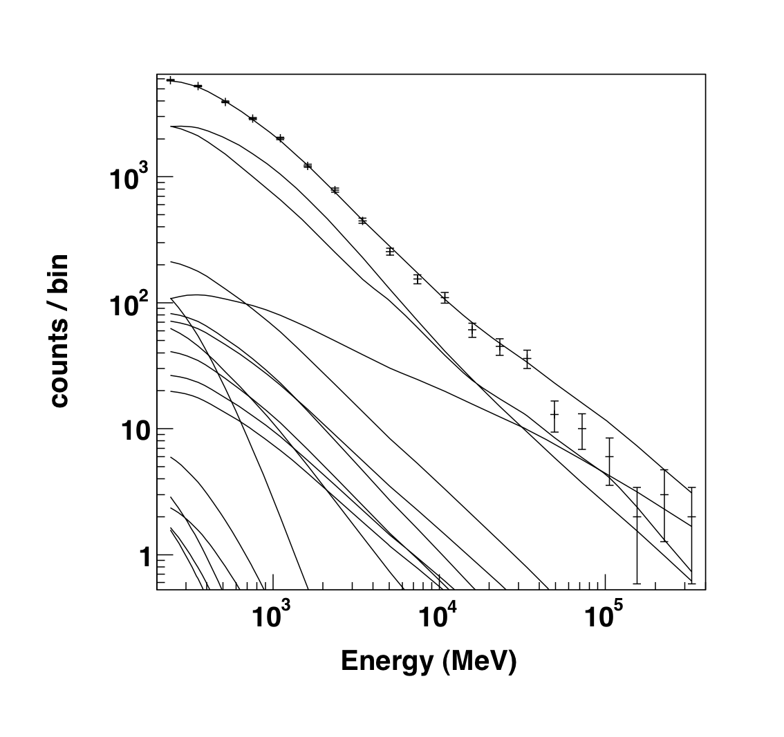
You can plot the results of the fit by executing the plot command. The results are shown below:
>>> like1.plot()
 |
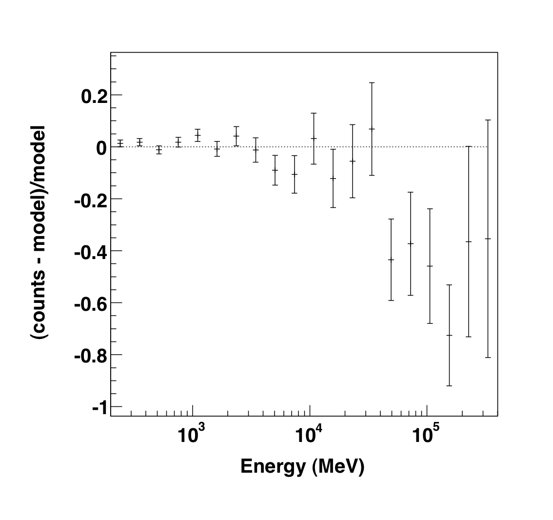 |
The output of the plot function of the like1 UnbinnedAnalysis object shows:
- Left: the contribution of each of the objects in the model to the total model, and plots the data points on top.
- Right: the residuals of the likelihood fit to the data.
We're already pretty close here (compare the Integral and Index of the above fit to those in the paper) but we want to continue to a finer fit tolerance and we'll need access to the covariance matrix for the next steps. First, save the results of this first fit to a file.
>>> like1.logLike.writeXml('PG1553_fit1.xml')
Now, create a new UnbinnedAnalysis object using the same UnbinnedObs object from before and the results of the previous fit and tell it to use the NewMinuit optimizer. We also double check that the tolerance is what we want (0.001) and then we fit the model making sure that we tell it we want it to compute the covariance matrix.
>>> like2 = UnbinnedAnalysis(obs,'PG1553_fit1.xml' ,optimizer='NewMinuit')

>>> like2.tol

0.001

>>> like2.fit(covar=True, verbosity=0)

>>> like2.model['_1FGLJ1555.7+1111']

_1FGLJ1555.7+1111

   Spectrum: PowerLaw2

33      Integral:  4.955e-01  2.999e-02  1.000e-04  1.000e+04 ( 1.000e-07)

34         Index:  1.671e+00  3.333e-02  0.000e+00  5.000e+00 (-1.000e+00)

35    LowerLimit:  2.000e+02  0.000e+00  3.000e+01  5.000e+05 ( 1.000e+00) fixed

36    UpperLimit:  4.000e+05  0.000e+00  3.000e+01  5.000e+05 ( 1.000e+00) fixed

>>> like2.logLike.writeXml('PG1553_fit2.xml')
The results of the final fit are slightly different than the previous fit and the errors are a bit better. You should double check your results to those here to make sure that nothing is off. If there's some large difference, go back through the thread and try to figure out where the deviation is. Don't forget to save the results to a file so we can use it in a bit. You can also get the TS value for a specific source:
>>> like2.Ts('_1FGLJ1555.7+1111')

2412.5434743046062
and if you import the math module you can calculate how many standard deviations (σ) this corresponds to. (Remember that the TS value is ∼ σ2.)
>>> import math

>>> math.sqrt( like2.Ts('_1FGLJ1555.7+1111') )

49.117649315746029
Create some TS Maps
We're going to deviate here a bit and go out of python to create two test statistic (TS) Maps. A TS map is created by moving a putative point source through a grid of locations on the sky and maximizing the log(likelihood) at each grid point. We could do this within python (via the TsMap object) but I think calling gttsmap from the command line is beneficial here. If you have access to multiple CPUs, you might want to start one of the maps running in one terminal and the other in another one since this will take several hours to complete. Our main goal is to create one TS Map with PG1553 included in the fit and another without. The first one will allow us to make sure we didn't miss any sources in our ROI and the other will allow us to see the source. All of the other sources in our model file will be included in the fit and shouldn't show up in the final map.
If you don't want to create these maps, go ahead and skip the following steps and jump to the section on making a butterfly plot. The creation of these maps is optional and is only for double checking your work. You should still modify your model fit file as detailed in the following paragraph.
First, modify PG1553_fit2.xml to make everything fixed by changing all of the free="1" statements to free="0". Modify the lines that look like:
<parameter error="1.670710816" free="1" max="10000" min="0.0001" name="Prefactor" scale="1e-13" value="6.248416874" /><
<parameter error="0.208035277" free="1" max="5" min="0" name="Index" scale="-1" value="2.174167564" />
to look like:
<parameter error="1.670710816" free="0" max="10000" min="0.0001" name="Prefactor" scale="1e-13" value="6.248416874" /><
<parameter error="0.208035277" free="0" max="5" min="0" name="Index" scale="-1" value="2.174167564" />
Also, change the integral and index parameter for 1FGLJ1555.7+1111 from free to fixed (remember we fit this with a powerlaw2 model and not a powerlaw model). Then copy it and call it PG1553_fit2_noPG1553.xml and comment out (or delete) the PG1553 source. If you want to generate the TS maps, in one window do the following:
[user@localhost]$ gttsmap

Event data file[] PG1553_filtered_gti.fits

Spacecraft data file[] SC.fits

Exposure map file[none] expMap.fits

Exposure hypercube file[none] expCube.fits

Source model file[] PG1553_fit2.xml

TS map file name[] PG1553_TSmap_resid.fits

Response functions to use[P6_V3_DIFFUSE] P6_V3_DIFFUSE

Optimizer (DRMNFB|NEWMINUIT|MINUIT|DRMNGB|LBFGS) [MINUIT] MINUIT

Fit tolerance[1e-05] 1e-05

Number of X axis pixels[] 25

Number of Y axis pixels[] 25

Image scale (in degrees/pixel)[] 0.5

Coordinate system (CEL|GAL) [CEL] CEL

X-coordinate of image center in degrees (RA or l)[] 238.929

Y-coordinate of image center in degrees (Dec or b)[] 11.1901

Projection method (AIT|ARC|CAR|GLS|MER|NCP|SIN|STG|TAN) [STG] STG
In another window do the following:
[user@localhost]$ gttsmap

Event data file[] PG1553_filtered_gti.fits

Spacecraft data file[] SC.fits

Exposure map file[none] expMap.fits

Exposure hypercube file[none] expCube.fits

Source model file[] PG1553_fit2_noPG1553.xml

TS map file name[] PG1553_TSmap_noPG1553.fits

Response functions to use[P6_V3_DIFFUSE] P6_V3_DIFFUSE

Optimizer (DRMNFB|NEWMINUIT|MINUIT|DRMNGB|LBFGS) [MINUIT] MINUIT

Fit tolerance[1e-05] 1e-05

Number of X axis pixels[] 25

Number of Y axis pixels[] 25

Image scale (in degrees/pixel)[] 0.5

Coordinate system (CEL|GAL) [CEL] CEL

X-coordinate of image center in degrees (RA or l)[] 238.929

Y-coordinate of image center in degrees (Dec or b)[] 11.1901

Projection method (AIT|ARC|CAR|GLS|MER|NCP|SIN|STG|TAN) [STG] STG
This will take a while (over 3 hours each) so go get a cup of coffee. The final TS maps will be pretty rough since we selected to only do 25x25 0.5 degree bins but it will allow us to check if anything is missing and go back and fix it. These rough plots aren't publication ready but they'll do in a pinch to verify that we've got the model right.
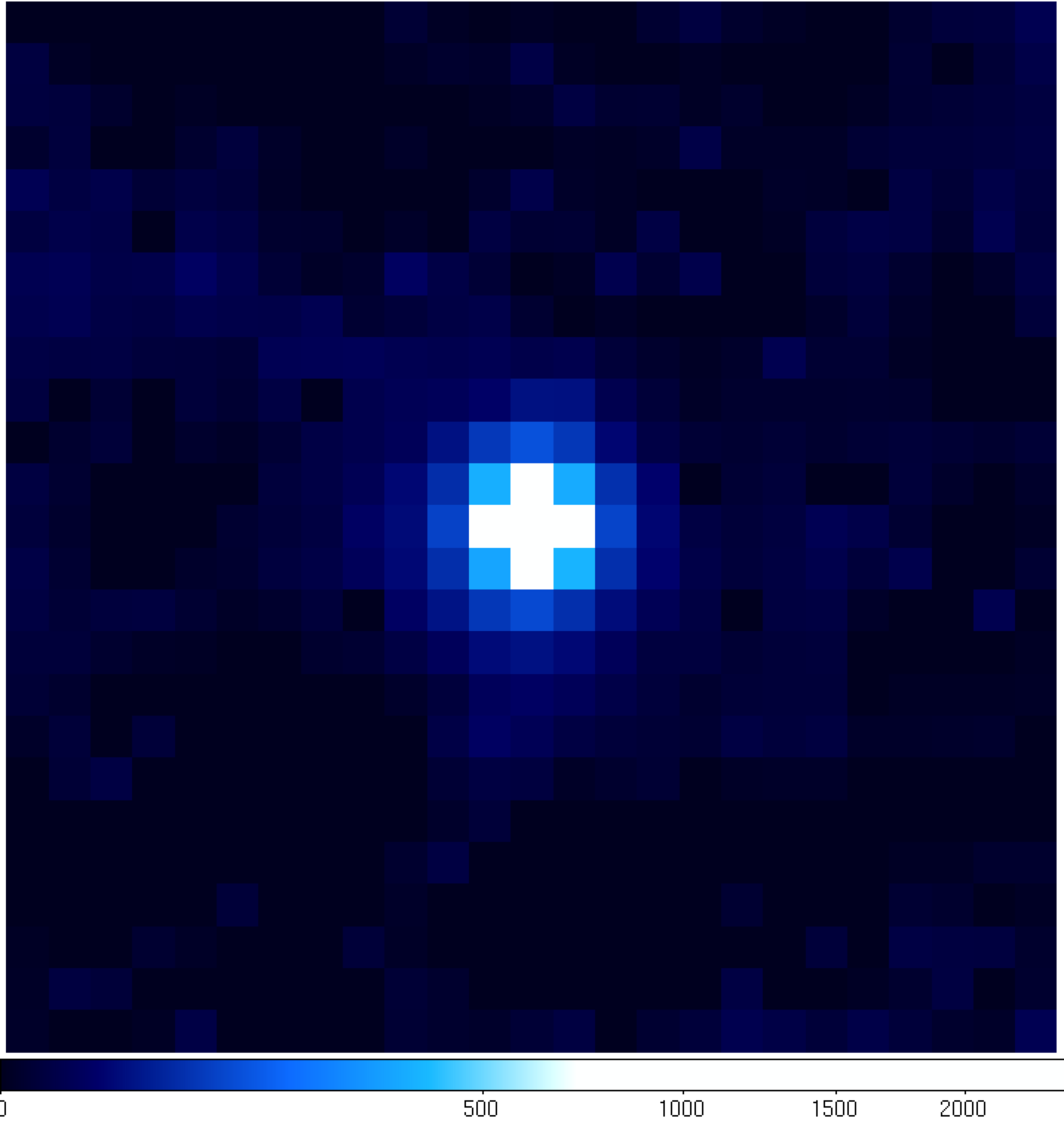
Once the TS maps have been generated, open them up in whatever viewing program you wish (we're using ds9 here).
 |
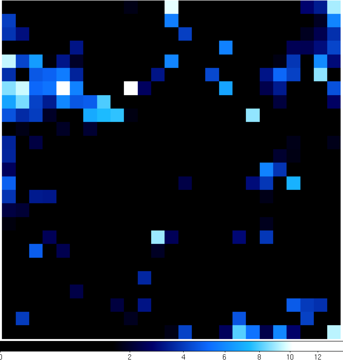 |
You can see that the 'noPG1553' map (left) has a prominent source in the middle of the ROI. This is PG 1553+113 and if you hover over the center pixel, the TS value of that pixel matches pretty well with the TS value of PG 1553+113 that we calculated within python. If you then open up the 'residuals' plot (right), you can see that it's pretty flat in TS space (the brightest pixel has a TS value of 14). This indicates that we didn't miss any significant sources. If you did see something significant (TS > 20 or so), you probably should go back and figure out what source you missed.
Produce the Butterfly Plot
Now we'll use the covariance matrix to calculate the decorrelation energy (the decorrelation energy is the energy at which the correlation between the flux normalization and spectral index is minimized) and the differential flux along with their errors, the first steps in producing a butterfly plot of the SED. We first need to find the correlation coefficients for the integral and index we fit in the above section. The descriptions of these variables are beyond the scope of this thread and can be found in the Cicerone.
To find the correlation coefficients we first need to find which column corresponds to which variable in the model in the list2.covariance matrix. The way to do this is to print out the model in python by calling like2.model and count down from the top (starting with zero) all of the free parameters until you get to those associated with PG 1553+113. You'll find that the Integral parameter (parameter 44) is the 10th free parameter and the Index is the 11. To verify:
>>> math.sqrt(like2.covariance[10][10])

0.029988497540106664

>>> math.sqrt(like2.covariance[11][11])

0.033333799524015592
Since covγγ = σγ2 and covII = σI2 (where σ is the spectral index and I is the integral flux) these numbers should match the error listed when you call like2.model['_1FGLJ1555.7+1111']. In this case they do and you can access the covariance between these two parameters:
>>> like2.covariance[10][11]

0.00057930603563618218

>>> like2.covariance[11][10]

0.00057930603563618218
These are the same since covγI = covIγ. In this same way, you can get the covariance values for any of the parameters in the covariance matrix. Note that you could write up a quick algorithm that'll find these parameters for you but you've probably guessed that such a function exists in the likeSED.py module and we'll be using that in a bit.
Calculate Decorrelation Energy
The decorrelation energy can be calculated using the following formula (note that the derivation and explanation of this can be found in the Cicerone).
![]()
where E1 and E2 are the LowerLimit and UpperLimit of the model respectively, ε is (E2/E1)1+γ and γ is negative. So, let's calculate this number along with some sanity checks:
>>> E1 = like2.model['_1FGLJ1555.7+1111'].funcs['Spectrum']. getParam('LowerLimit').value()

>>> E2 = like2.model['_1FGLJ1555.7+1111'].funcs['Spectrum']. getParam('UpperLimit').value()

>>> gamma = like2.model['_1FGLJ1555.7+1111'].funcs['Spectrum']. getParam('Index').value()

>>> I = like2.model['_1FGLJ1555.7+1111'].funcs['Spectrum']. getParam('Integral').value()

>>> cov_gg = like2.covariance[11][11]

>>> cov_II = like2.covariance[10][10]

>>> cov_Ig = like2.covariance[10][11]

>>> print "Index: " + str(gamma) + " +/- " + str(math.sqrt(cov_gg))

Index: 1.67115136208 +/- 0.033333799524

>>> print "Integral: " + str(I) + " +/- " + str(math.sqrt(cov_II))

Integral: 0.495514212298 +/- 0.0299884975401

>>> print E1,E2

200.0 400000.0

>>> epsilon = (E2/E1)**(1-gamma)

>>> logE0 = (math.log(E1) - epsilon*math.log(E2))/(1-epsilon) + 1/(gamma-1) + cov_Ig/(I*cov_gg)

>>> E0 = math.exp(logE0)

>>> print E0

2420.92968133
This final number is in whatever units E1 and E2 were in (in this case, MeV).
Calculate the Differential Flux
Now that we have the decorrelation energy we can calculate the differential flux pre-factor and the error. You could go back and refit the data using a PowerLaw model which gives this value out to you but we've got all the numbers in front of us to do it right away.
![]()
where X1 =E1/E0 and X2 = E2/E0.
>>> X1 = E1/E0

>>> X2 = E2/E0

>>> N0 = I/(E0*((X1**(1-gamma) - X2**(1-gamma)) / (gamma - 1)))

>>> print N0

2.5925184974e-05
and the error on the differential flux is:
![]()
where
![]()
>>> rho_sq = cov_Ig**2/(cov_II*cov_gg)

>>> N0_err = N0 * math.sqrt(cov_II) * math.sqrt(1 - rho_sq) / I

>>> print N0_err

1.27988104258e-06
Calculate the Butterfly Plot
We need to calculate the differential flux at several energy points as well as the error on that differential flux. The differential flux is defined as:
![]()
and the error on that flux is defined as:
![]()
So, let run a quick loop to calculate F(E) and F(E) +/- Δ F(E) so that we can plot it. It might be easier to copy all of this to a file and run it as a python script. The following python commands will output the results to a file called butterfly.txt.
>>> def calcF(E,N0,E0,gamma):

Note the indentation (space) of the following lines.

... F = N0*(E/E0)**(-1*gamma)

... return F

...

>>> def calcFerr(E,F,N0,N0err,E0,cov_gg):

Note the indentation (space) of the following lines.

... Ferr = F*math.sqrt(N0err**2/N0**2 + ((math.log(E/E0))**2)*cov_gg)

... return Ferr

...

>>> file = open("butterfly.txt", "w")

>>> E = 200

>>> while(E<200000):

Note the indentation (space) of the following lines.

... F = calcF(E,N0,E0,gamma)

... Ferr = calcFerr(E,F,N0,N0_err,E0,cov_gg)

... print >>file, E,F,Ferr

... E+=100

...

>>> file.close()
You can now plot these data with your favorite plotter to get the final butterfly plot. The first column is the
energy (in MeV), the second is the best fit line and the last is the error on that best fit line at that energy. You
should plot a line above the best fit line by adding the second and third columns and then a line below the best fit
line by subtracting the third column from the second column. Note that the spread of the butterfly is smaller here
than in the published result because the systematic error on the differential flux and spectral index are included in
their result. If you add in these systematic uncertainties when you are calculating the values above, your butterfly
will more closely match those obtained in the paper. Here I used gnuplot with the following commands to produce the butterfly diagram below.
(
[user@localhost]$ gnuplot


	G N U P L O T

	Version 4.4 patchlevel 2

	last modified Wed Sep 22 12:10:34 PDT 2010

	System: Darwin 10.6.0


	Copyright (C) 1986-1993, 1998, 2004, 2007-2010

	Thomas Williams, Colin Kelley and many others


	gnuplot home:     http://www.gnuplot.info

	faq, bugs, etc:   type "help seeking-assistance"

	immediate help:   type "help"

	plot window:      hit 'h'


Terminal type set to 'aqua'

gnuplot> set log y

gnuplot> set log x

gnuplot> p 'butterfly.txt' u 1:($2+$3):($2-$3) w filledcurves
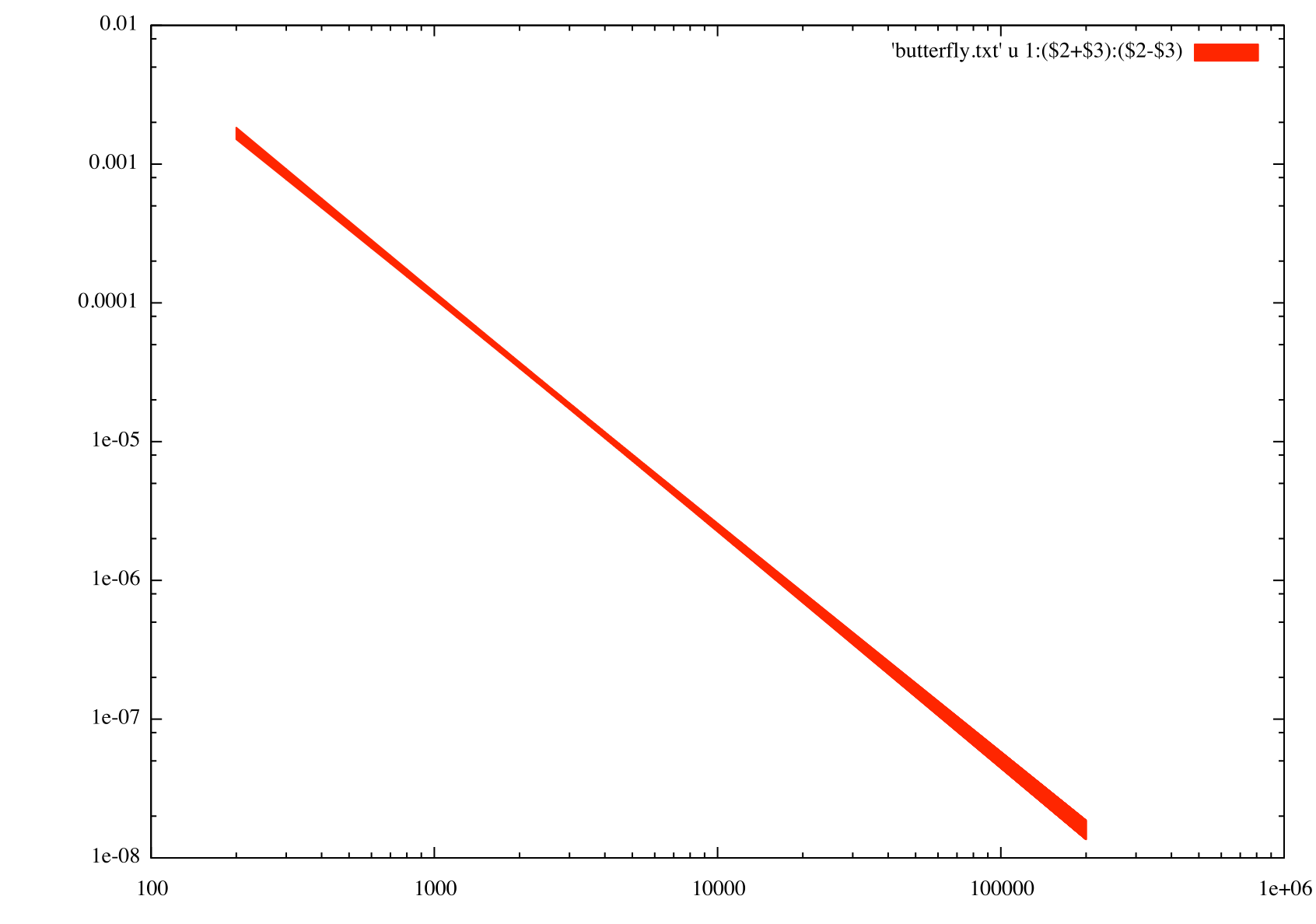
Generate Spectral Points
To generate spectral points to plot on top of the butterfly that we just produced, you need to go back to the data selection part and use gtselect (filter in python) to divide up your data set in energy bins and run the likelihood fit on each of these individual bins. Luckily, there's a script that does this for us that we'll employ to get a final result. This script also generates the butterfly plot we just produced so you won't have to redo that again and it also does a lot of checks on the data to make sure that everything is going ok. If you've made it this far, you might be a little curious as to why we didn't jump right into using this tool but now you're in a position to play with the python tools and make them do what you want them too (and the script doesn't have the ability to calculate the decorrelation energy). The script is also much more careful in handling units and saving everything to files than we have been in this interactive session.
So download the likeSED.py user contributed tool (it's in the SED_scripts package) and load it up into python. You can find information on the usage of this tool on the same page where you downloaded it. It can be used to generate an SED plot for both binned and unbinned analyses but we're only going to work on a binned analysis here.
>>> from likeSED import *

This is likeSED version 10.
Now you need to create a likeInput object that takes our unbinnedAnalysis object, the source name and the number of bins we want as arguments. We're going to make 9 bins here like in the paper and we're also going to make custom bins and bin centers. You can have the module chose bins and bin centers for you (via the getECent function) but we're going to do it this way so we can have the double-wide bin at the end. We're also going to use the 'fit2' file (the result of our fit on the full dataset with the NewMinuit optimizer) for the fits of the individual bins but we need to edit it first to make everything fixed except for the integral value of PG 1553+113. Go ahead and do that now. We're basically assuming that the spectral index is the same for all bins and that the contributions of the other sources within the ROI are not changing with energy.
>>> inputs = likeInput(like2,'_1FGLJ1555.7+1111',nbins=9, model='PG1553_fit2.xml')

>>> low_edges = [200.,427.69,914.61,1955.87,4182.56,8944.27,19127.05,40902.61]

>>> high_edges = [427.69,914.61,1955.87,4182.56,8944.27,19127.05,40902.61,187049.69]

>>> centers = [0.2767, 0.5917, 1.265, 2.706, 5.787, 12.37, 26.46, 86.60]

>>> inputs.customBins(low_edges,high_edges)
This last step will take a while (approximately 10 minutes) because it's creating an expmap and event file for each of the bins that we requested (look in your working directory for these files). Once it is done we'll tell it to do the fit of the full energy band and make sure we request that it keep the covariance matrix. Then we'll create a likeSED object from our inputs, tell it where we want our centers to be and then fit each of the bands. After this is done, we can plot it all with the Plot function.
>>> inputs.fullFit(CoVar=True)

Full energy range model for _1FGLJ1555.7+1111:

_1FGLJ1555.7+1111

Spectrum: PowerLaw2

33      Integral:  4.955e-01  2.999e-02  1.000e-04  1.000e+04 ( 1.000e-07)

34         Index:  1.671e+00  3.333e-02  0.000e+00  5.000e+00 (-1.000e+00)

35    LowerLimit:  2.000e+02  0.000e+00  3.000e+01  5.000e+05 ( 1.000e+00) fixed

36    UpperLimit:  4.000e+05  0.000e+00  3.000e+01  5.000e+05 ( 1.000e+00) fixed


Flux 0.2-400.0 GeV 5.0e-08 +/- 3.0e-09 cm^-2 s^-1

Test Statistic 2412.53719993

>>> sed = likeSED(inputs)

>>> sed.customECent(centers)

>>> sed.fitBands()

-Running Likelihood for band0-

-Running Likelihood for band1-

-Running Likelihood for band2-

-Running Likelihood for band3-

-Running Likelihood for band4-

-Running Likelihood for band5-

-Running Likelihood for band6-

-Running Likelihood for band7-

>>> sed.Plot()
This produces the following three plots: a TS plot, a counts spectrum, and a butterfly plot (statistical errors only):
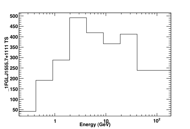
The TS plot shows the TS value for each bin in the spectrum produced by likeSED. Notice that the last bin is double-wide.
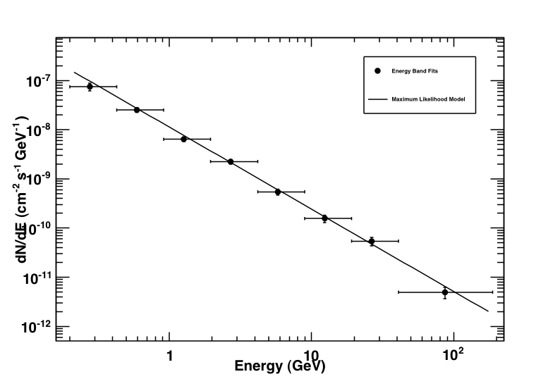
Counts spectrum produced by likeSED along with the spectral points.
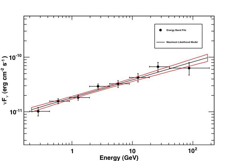
Butterfly plot along with the spectral points produced by likeSED. Note that this plot does not include the systematic errors.
Now we're going to leave python and look at the files that likeSED produced. In your working directory you will find a bunch of _1FGLJ1555.7+1111_9bins_custom files. These are just the event and exposure maps for each bin we selected. If you wanted to completely redo the likeSED analysis you should delete these. Some other files to note are _1FGLJ1555.7+1111_9bins_custom_likeSEDout.fits which contains all of the data needed to reproduce the plots seen when we ran the Plot function. There is also a root file (_1FGLJ1555.7+1111_9bins_custom_histos.root) with dumps of the plots and eps files of all of the plots. Now that we've generated a butterfly SED and individual SED data points we can move on to working on a light curve.
Building a Light Curve
The process for producing a light curve is pretty simple. We take the model fit we have (the fit2 file) and set all parameters to fixed except the index and Integral of PG 1553+113, generate an event file for a single time bin, run gtmktime, generate an exposure cube and exposure map for that time bin and run the likelihood on that and get out the integral and index for that bin. In the paper, they did this for 2-day bins but we'll make weekly 7 day bins here just to make our job a bit easier and faster. You could also generate a light curve via Aperture Photometry which is much quicker but less rigorous. There is also a perl script in the user contributed tools that will generate lightcurves which you could use here.
Here's the final script that should do what we want it to do: light_curve.py. Note that this script is not completely rigorous and not suited to generate scientific results but it'll get us going in the right direction.
Open the file up in your favorite text editor and have a look at what we're going to do. We first do a loop over the data and calculate an event file, an exposure map and cube for each iteration and then run pyLikelihood on those files. Notice that we put all of the variables we wanted from the fit up in a python list and that we just print these out at the end. The script should take about 30 minutes to run and it saves the results to a file called "light_curve.txt". The output from this script should look a bit like this (for one step):
>>> from light_curve import *

**Working on range (239557417,240162217)**


***Running gtselect***

time -p ~/ScienceTools/i386-apple-darwin10.4.0/bin/gtselect infile=PG1553_filtered.fits outfile=LC_PG1553_filtered_bin0.fits ra=238.929 dec=11.1901 rad=10.0 tmin=239557417.0 tmax=240162217.0 emin=200.0 emax=400000.0 zmax=105.0 evclsmin=3 evclsmax=4 evclass="INDEF" convtype=-1 phasemin=0.0 phasemax=1.0 evtable="EVENTS" chatter=2 clobber=yes debug=no gui=no mode="ql"

Done.

real 3.17

user 0.20

sys 0.08

***Running gtmktime***

time -p ~/ScienceTools/i386-apple-darwin10.4.0/bin/gtmktime scfile=SC.fits sctable="SC_DATA" filter="(DATA_QUAL==1)&&(LAT_CONFIG==1)&&ABS(ROCK_ANGLE)<52" roicut=yes evfile=LC_PG1553_filtered_bin0.fits evtable="EVENTS" outfile="LC_PG1553_filtered_gti_bin0.fits" apply_filter=yes overwrite=no header_obstimes=yes tstart=0.0 tstop=0.0 gtifile="default" chatter=2 clobber=yes debug=no gui=no mode="ql"

real 0.79

user 0.33

sys 0.08

***Running gtltcube***

time -p ~/ScienceTools/i386-apple-darwin10.4.0/bin/gtltcube evfile="LC_PG1553_filtered_gti_bin0.fits" evtable="EVENTS" scfile=SC.fits sctable="SC_DATA" outfile=LC_expCube_bin0.fits dcostheta=0.025 binsz=1.0 phibins=0 tmin=0.0 tmax=0.0 file_version="1" zmax=180.0 chatter=2 clobber=yes debug=no gui=no mode="ql"

Working on file SC.fits

.....................!

real 57.41

user 54.19

sys 0.70

***Running gtexpmap***

time -p ~/ScienceTools/i386-apple-darwin10.4.0/bin/gtexpmap evfile=LC_PG1553_filtered_gti_bin0.fits evtable="EVENTS" scfile=SC.fits sctable="SC_DATA" expcube=LC_expCube_bin0.fits outfile=LC_expMap_bin0.fits irfs="P6_V3_DIFFUSE" srcrad=20.0 nlong=120 nlat=120 nenergies=20 submap=no nlongmin=0 nlongmax=0 nlatmin=0 nlatmax=0 chatter=2 clobber=yes debug=no gui=no mode="ql"

The exposure maps generated by this tool are meant

to be used for *unbinned* likelihood analysis only.

Do not use them for binned analyses.

Computing the ExposureMap using LC_expCube_bin0.fits

....................!

real 88.86

user 85.68

sys 0.67

***Running likelihood analysis***


...The output from the calculations of the other bins will be here...
Once the script completes, you can plot these data using your favorite plotting tool. I used the following commands to produce the following two figures with gnuplot:
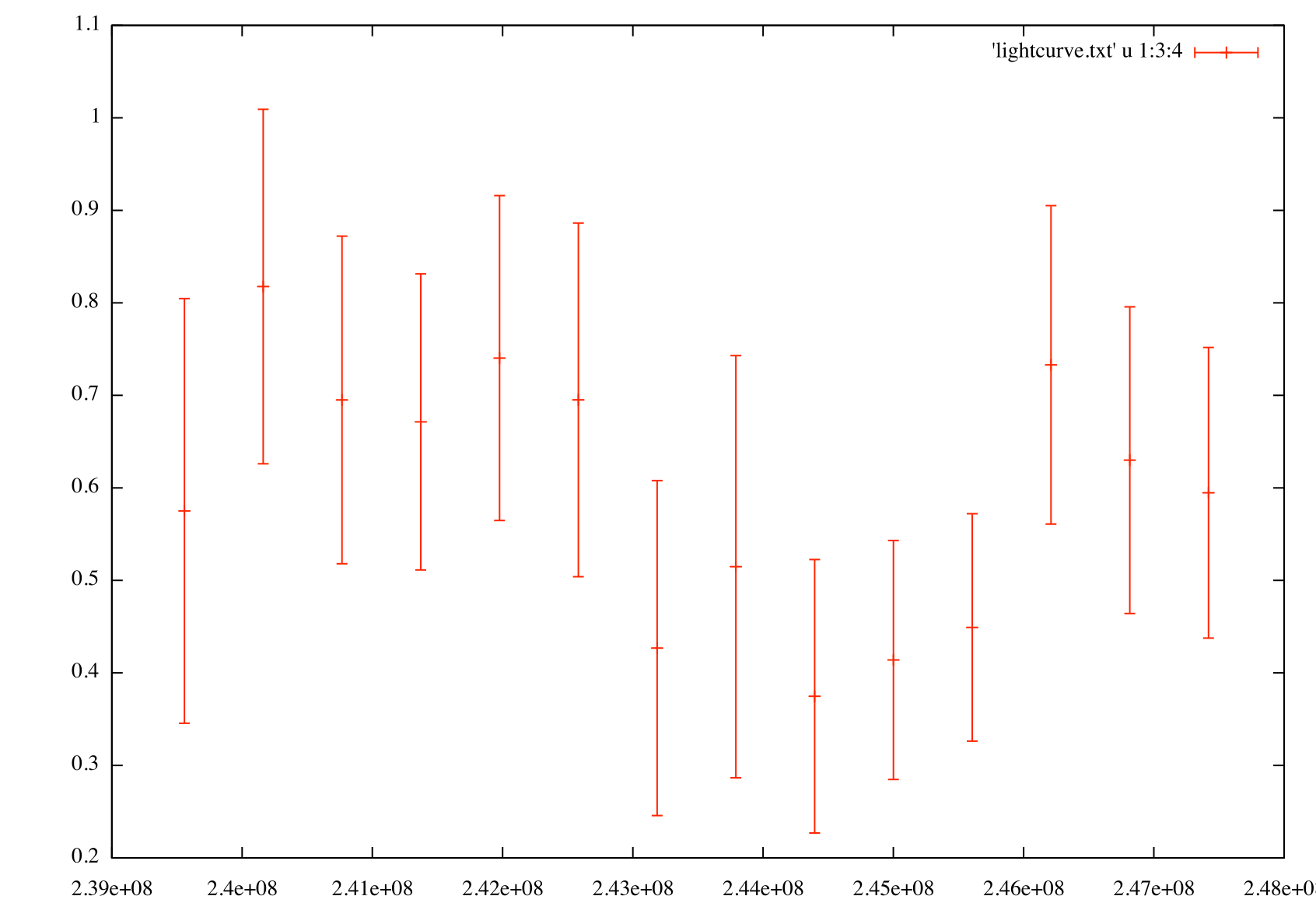
Generate a flux light curve

gnuplot> p 'light_curve.txt' u 1:3:4 w yerr

Generate an index light curve

gnuplot> p 'light_curve.txt' u 1:5:6 w yerr
 |
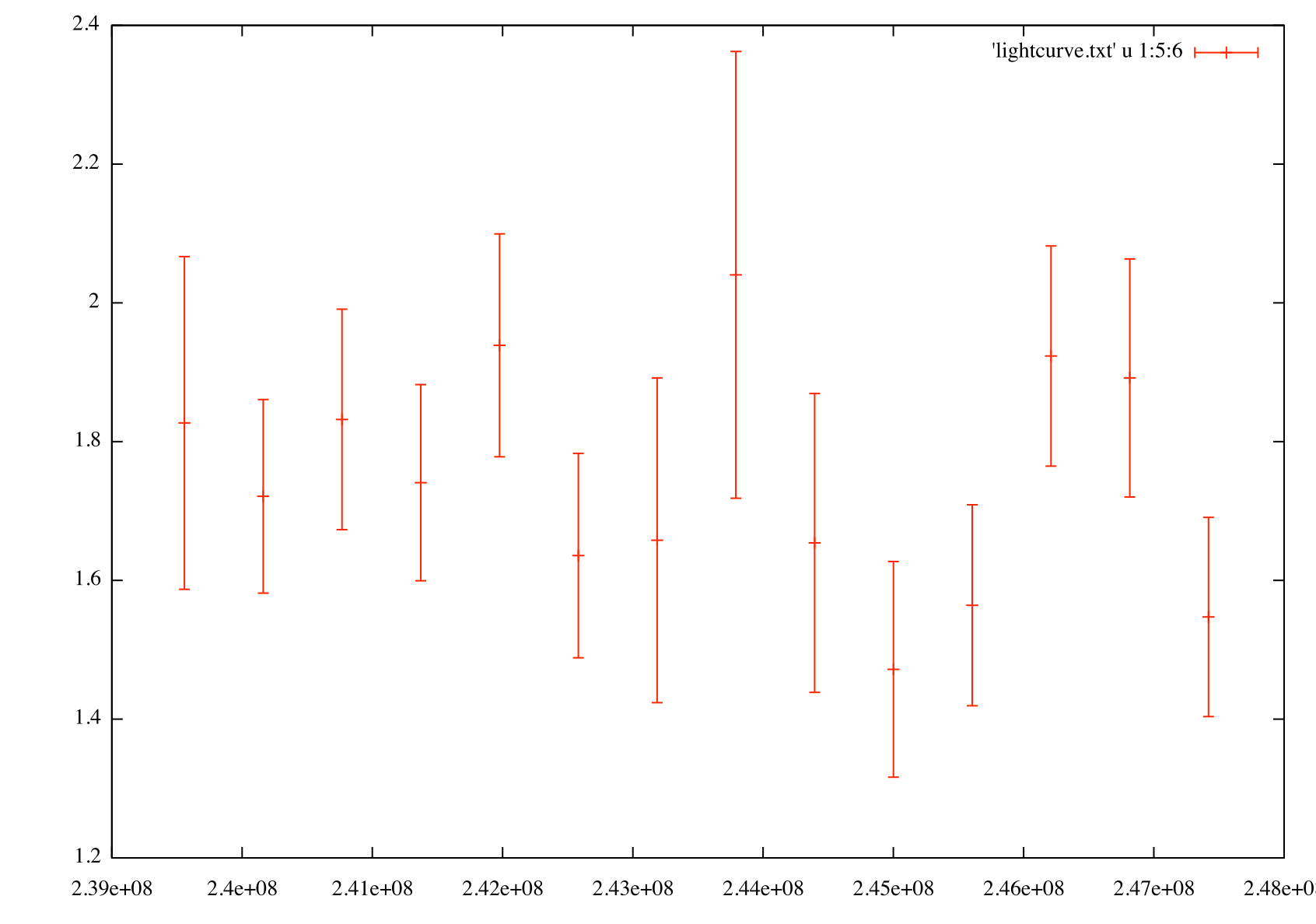 |
The flux light curve (left) shows flux vs. time for PG 1553+113 in weekly bins. The index light curve (right) shows spectral index vs. time for PG 1553+113 in weekly bins.
Upper Limits
One thing you might want to do is to make one of the data points into an upper limit instead of an actual data point. Since we've increased the width of these bins from the paper you can see that we've got good statistics for each of the bins (look at the TS values in the output file of the light curve script) but we'll take the bin with the smallest TS value (bin 7 at MET 243791017 has a TS value of 27.4, it's the one with the largest error bars in the spectral index light curve) and calculate an upper limit for it. This exact same method would work if you were perfoming a binned analysis.
>>> obs = UnbinnedObs('LC_PG1553_filtered_gti_bin7.fits', 'SC.fits', expMap='LC_expMap_bin7.fits',
expCube='LC_expCube_bin7.fits', irfs='P6_V3_DIFFUSE')

>>> like = UnbinnedAnalysis(obs,'PG1553_fit2.xml',optimizer='NewMinuit')

>>> like.fit(verbosity=0,covar=True)

6738.4636761507745

>>> like.Ts('_1FGLJ1555.7+1111')

27.413823645321827

>>> from UpperLimits import UpperLimits

>>> ul=UpperLimits(like)

>>> ul['_1FGLJ1555.7+1111'].compute()

0 0.517996435127 2.71065800916e-08 1.07099361372e-07

1 0.609550868982 0.075223923026 1.32933210228e-07

2 0.701105302838 0.282231188434 1.60344777593e-07

3 0.792659736693 0.600753399523 1.89163817121e-07

4 0.884214170549 1.01577008582 2.19540840456e-07

5 0.959945239685 1.42361237188 2.45904837617e-07

(2.4146955358835266e-07, 0.94720480433553234)

>>> ul['_1FGLJ1555.7+1111'].results

[2.41e-07 ph/cm^2/s for emin=100.0, emax=300000.0, delta(logLike)=1.35]
If we were smart going in, we would have included this step in each calculation of the light curve above so that we wouldn't have to go back and do this (or be even more intelligent and check for a low TS value). Notice that this upper limit is for 100 to 300000 MeV which is probably not what we want since we're only looking at values above 200 MeV. Let's go back and fix this:
>>> ul['_1FGLJ1555.7+1111'].compute(emin=200,emax=4e5)

0 0.517996435127 2.71065800916e-08 5.19578943608e-08

1 0.609550868982 0.075223923026 6.11531729198e-08

2 0.701105302838 0.282231188434 7.0350869324e-08

3 0.792659736693 0.600753399523 7.95506508327e-08

4 0.884214170549 1.01577008582 8.87527182072e-08

5 0.959945239685 1.42361237188 9.63661743282e-08

(9.5085342740784354e-08, 0.94720480433553234)

>>> ul['_1FGLJ1555.7+1111'].results

[2.41e-07 ph/cm^2/s for emin=100.0, emax=300000.0, delta(logLike)=1.35,9.51e-08 ph/cm^2/s for emin=200.0, emax=400000.0, delta(logLike)=1.35]
The results are in a python list and it keeps track of all the upper limits you've computed. Now you can use this upper limit in your light curve if you so choose. This method can also be used to calculate an upper limit on the full data set if you are analyzing a non-detectable source.
Finished
So, it looks like we've reproduced all of the results in the PG 1553+113 paper. I hope that you have a better idea of what you can do with the python tools and the likeSED script. This tutorial should be a jumping off point into writing your own analysis scripts.
Last updated by: Jeremy S. Perkins 04/11/2011