National Aeronautics and Space Administration

Goddard Space Flight Center

Data

• Data Policy
• Data Access
• Data Analysis

• Caveats
• Newsletters
• FAQ

Likelihood Analysis with Python

The python likelihood tools are a very powerful set of analysis tools that expand upon the command line tools provided with the Fermi Science Tools package. Not only can you perform all of the same likelihood analysis with the python tools that you can with the standard command line tools but you can directly access all of the model parameters. You can more easily script a standard analysis like light curve generation. There are also a few things built into the python tools that are not available from the command line like the calculation of upper limits.

There are many user contributed packages built upon the python backbone of the Science Tools and we are going to highlight and use a few of them in this tutorial like likeSED, make2FGLxml, and the LATAnalysisScripts.

This sample analysis is based on the PG 1553+113 analysis performed by the LAT team and described in Abdo, A. A. et al. 2010, ApJ, 708, 1310. At certain points we will refer to this article as well as the Cicerone. After you complete this tutorial you should be able to reproduce all of the data analysis performed in this publication including generating a spectrum (individual bins and a butterfly plot) and produce a light curve with the python tools. This tutorial assumes you have the most recent ScienceTools installed. We will also make significant use of python, so you might want to familiarize yourself with python (there's a beginner's guide at http://wiki.python.org/moin/BeginnersGuide). This tutorial also assumes that you've gone through the non-python based unbinned likelihood thread. This tutorial should take approximately 8 hours to complete (depending on your computer's speed) if you do everything but there are some steps you can skip along the way which shave off about 4 hours of that.

Note: In this tutorial, commands that start with '[user@localhost]$' are to be executed within a shell environment (bash, c-shell etc.) while commands that start with '>>>' are to be executed within an interactive python environment. Commands are in bold and outputs are in normal font. Text in ITALICS within the boxes are comments from the author.

Get the Data

For this thread the original data were extracted from the LAT data server with the following selections (these selections are similar to those in the paper):

• Search Center (RA,Dec) = (238.929,11.1901)
• Radius = 20 degrees
• Start Time (MET) = 239557417 seconds (2008-08-04T15:43:37)
• Stop Time (MET) = 256970880 seconds (2009-02-22T04:48:00)
• Minimum Energy = 100 MeV
• Maximum Energy = 300000 MeV

We've provided direct links to the event files as well as the spacecraft data file if you don't want to take the time to use the download server. For more information on how to download LAT data please see the Extract LAT Data tutorial. Note that these data files were created on April 22, 2014 and might not work with the most up-to-date version of the tools. If you run into issues, use the data server to download new files.

• L1405021409359D489E7F83_PH00.fits
• L1405021409359D489E7F83_PH01.fits
• L1405021409359D489E7F83_SC00.fits

You'll first need to make a file list with the names of your input event files:

[user@localhost]$ ls -1 *PH*.fits > PG1553_events.list

In the following analysis we've assumed that you've named your list of data files PG1553_events.list and the spacecraft file PG1553_SC.fits.

Perform Event Selections

You could follow the unbinned likelihood tutorial to perform your event selections using gtlike, gtmktime etc. directly from the command line, and then use pylikelihood later. But we're going to go ahead and use python. The gt_apps module provides methods to call these tools from within python. This'll get us used to using python.

So, let's jump into python:

[user@localhost]$ python
Python 2.7.2 (default, Mar 30 2012, 18:13:17)
[GCC 4.1.2 20080704 (Red Hat 4.1.2-50)] on linux2
Type "help", "copyright", "credits" or "license" for more information.
>>>


Ok, we want to run gtselect inside but we first need to import the gt_apps module to gain access to it.

>>> import gt_apps as my_apps

Now, you can see what objects are part of the gt_apps module by executing

>>> help(my_apps)


Which brings up the help documentation for that module (type 'x' to exit). The python object for gtselect is called filter and we first need to set all of it's options. This is very similar to calling gtselect form the command line and inputting all of the variables interactively. It might not seem that convenient to do it this way but it's really nice once you start building up scripts (see Building a Light Curve) and reading back options and such. For example, towards the end of this thread, we'll want to generate a light curve and we'll have to run the likelihood analysis for each datapoint. It'll be much easier to do all of this within python and change the tmin and tmax in an iterative fashion. Note that these python objects are just wrappers for the standalone tools so if you want any information on their options, see the corresponding documentation for the standalone tool.

>>> my_apps.filter['evclass'] = 2
>>> my_apps.filter['ra'] = 238.929
>>> my_apps.filter['dec'] = 11.1901
>>> my_apps.filter['rad'] = 10
>>> my_apps.filter['emin'] = 100
>>> my_apps.filter['emax'] = 300000
>>> my_apps.filter['zmax'] = 100
>>> my_apps.filter['tmin'] = 239557417
>>> my_apps.filter['tmax'] = 256970880
>>> my_apps.filter['infile'] = '@PG1553_events.list'
>>> my_apps.filter['outfile'] = 'PG1553_filtered.fits'


Once this is done, run gtselect:

>>> my_apps.filter.run()
time -p ~ScienceTools/x86_64-unknown-linux-gnu-libc2.5/bin/gtselect infile=@PG1553_events.list outfile=PG1553_filtered.fits ra=238.929 dec=11.1901 rad=10.0 tmin=239557417.0 tmax=256970880.0 emin=200.0 emax=300000.0 zmax=100.0 evclsmin="INDEF" evclsmax="INDEF" evclass=2 convtype=-1 phasemin=0.0 phasemax=1.0 evtable="EVENTS" chatter=2 clobber=yes debug=no gui=no mode="ql"
Done.
real 0.73
user 0.48
sys 0.10


Note that you can see exactly what gtselect will do if you run it by typing:

>>> my_apps.filter.command()
'time -p ~/ScienceTools/x86_64-unknown-linux-gnu-libc2.5/bin/gtselect infile=@PG1553_events.list outfile=PG1553_filtered.fits ra=238.929 dec=11.1901 rad=10.0 tmin=239557417.0 tmax=256970880.0 emin=200.0 emax=300000.0 zmax=100.0 evclsmin="INDEF" evclsmax="INDEF" evclass=2 convtype=-1 phasemin=0.0 phasemax=1.0 evtable="EVENTS" chatter=2 clobber=yes debug=no gui=no mode="ql"'


You have access to any of the inputs by directly accessing the filter['OPTIONS'] options.

Next, you need to run gtmktime. This is accessed within python via the maketime object:

>>> my_apps.maketime['scfile'] = 'PG1553_SC.fits'
>>> my_apps.maketime['filter'] = '(DATA_QUAL>0)&&(LAT_CONFIG==1)'
>>> my_apps.maketime['roicut'] = 'yes'
>>> my_apps.maketime['evfile'] = 'PG1553_filtered.fits'
>>> my_apps.maketime['outfile'] = 'PG1553_filtered_gti.fits'
>>> my_apps.maketime.run()
time -p ~/ScienceTools/x86_64-unknown-linux-gnu-libc2.5/bin/gtmktime scfile=SC.fits sctable="SC_DATA" filter="(DATA_QUAL>0)&&(LAT_CONFIG==1)" roicut=yes evfile=PG1553_filtered.fits evtable="EVENTS" outfile="PG1553_filtered_gti.fits" apply_filter=yes overwrite=no header_obstimes=yes tstart=0.0 tstop=0.0 gtifile="default" chatter=2 clobber=yes debug=no gui=no mode="ql"
real 2.85
user 2.61
sys 0.17


We're using the most conservative and most commonly used cuts described in deatil in the Cicerone.

Livetime Cubes and Exposure Maps

At this point, you could make a counts map of the events we just selected using gtbin (it's called evtbin within python) and I won't discourage you but we're going to go ahead and create a livetime cube and exposure map. This might take a few minutes to complete so if you want to create a counts map and have a look at it, get these processes going and open another terminal to work on your counts map (see the likelihood tutorial for an example of running gtbin to produce a counts map).

Livetime Cube

This step will take approximately 15 - 30 minutes to complete so if you want to just download the PG1553_ltCube from us you can skip this step.

>>> my_apps.expCube['evfile'] = 'PG1553_filtered_gti.fits'
>>> my_apps.expCube['scfile'] = 'PG1553_SC.fits'
>>> my_apps.expCube['outfile'] = 'PG1553_ltCube.fits'
>>> my_apps.expCube['dcostheta'] = 0.025
>>> my_apps.expCube['binsz'] = 1
>>> my_apps.expCube.run()
time -p ~/ScienceTools/x86_64-unknown-linux-gnu-libc2.5/bin/gtltcube evfile="PG1553_filtered_gti.fits" evtable="EVENTS" scfile=SC.fits sctable="SC_DATA" outfile=PG1553_ltCube.fits dcostheta=0.025 binsz=1.0 phibins=0 tmin=0.0 tmax=0.0 file_version="1" zmax=180.0 chatter=2 clobber=yes debug=no gui=no mode="ql"
Working on file PG1553_SC.fits
.....................!
real 2022.25
user 2018.97
sys 2.23


While you're waiting, you might have noticed that not all of the command line science tools have an equivalent object in gt_apps. This is easy to fix. Say you want to use gtltcubesun from within python. Just make it a GtApp:

>>> from GtApp import GtApp
>>> expCubeSun = GtApp('gtltcubesun','Likelihood')
>>> expCubeSun.command()
time -p ~/x86_64-unknown-linux-gnu-libc2.12/bin/gtltcubesun evfile="" evtable="EVENTS" scfile= sctable="SC_DATA" outfile=expCube.fits body="SUN" dcostheta=0.025 thetasunmax=180.0 binsz=0.5 phibins=0 tmin=0.0 tmax=0.0 powerbinsun=2.7 file_version="1" zmax=180.0 chatter=2 clobber=yes debug=no gui=no mode="ql"


Exposure Map

>>> my_apps.expMap['evfile'] = 'PG1553_filtered_gti.fits'
>>> my_apps.expMap['scfile'] ='PG1553_SC.fits'
>>> my_apps.expMap['expcube'] ='PG1553_ltCube.fits'
>>> my_apps.expMap['outfile'] ='PG1553_expMap.fits'
>>> my_apps.expMap['irfs'] ='CALDB'
>>> my_apps.expMap['srcrad'] =20
>>> my_apps.expMap['nlong'] =120
>>> my_apps.expMap['nlat'] =120
>>> my_apps.expMap['nenergies'] =20
>>> my_apps.expMap.run()
time -p ~/ScienceTools/x86_64-unknown-linux-gnu-libc2.5/bin/gtexpmap evfile=PG1553_filtered_gti.fits evtable="EVENTS" scfile=SC.fits sctable="SC_DATA" expcube=PG1553_ltCube.fits outfile=PG1553_expMap.fits irfs="CALDB" srcrad=20.0 nlong=120 nlat=120 nenergies=20 submap=no nlongmin=0 nlongmax=0 nlatmin=0 nlatmax=0 chatter=2 clobber=yes debug=no gui=no mode="ql"
The exposure maps generated by this tool are meant
to be used for *unbinned* likelihood analysis only.
Do not use them for binned analyses.
Computing the ExposureMap using PG1553_ltCube.fits
....................!
real 348.94
user 346.99
sys 0.51


Generate XML Model File

We need to create an XML file with all of the sources of interest within the Region of Interest (ROI) of PG 1553+113 so we can correctly model the background. For more information on the format of the model file and how to create one, see the likelihood analysis tutorial. We'll use the user contributed tool make2FGLxml.py to create a template based on the LAT 2-year catalog. You'll need to download the FITS version of this file at http://fermi.gsfc.nasa.gov/ssc/data/p7rep/access/lat/2yr_catalog/ and get the make2FGLxml.py tool from the user contributed software page. Also make sure you have the most recent galactic diffuse and isotropic model files which can be found at http://fermi.gsfc.nasa.gov/ssc/data/p7rep/access/lat/BackgroundModels.html.

Now that we have all of the files we need, you can generate your model file in python:

>>> from make2FGLxml import *
This is make2FGLxml version 04r1.
For use with the gll_psc_v02.fit and gll_psc_v05.fit and later LAT catalog files.
>>> mymodel = srcList('gll_psc_v08.fit','PG1553_filtered_gti.fits','PG1553_model.xml')
>>> mymodel.makeModel('gll_iem_v05_rev1.fit', 'gll_iem_v05_rev1', 'iso_source_v05_rev1.txt', 'iso_source_v05_rev1')
Creating file and adding sources for 2FGL
Added 24 point sources and 0 extended sources


For more information on the make2FGLxml module, see the usage notes. Note that we have named the isotropic diffuse model 'iso_source_v05' and not 'iso_source_v05_rev1'. The files associated with these two names (iso_source_v05.txt and iso_source_v05_rev1.txt) are identical but the diffuse column is named for the former and not the latter so we must match the column name in our model file. If you don't understand what was just said, don't worry about it.

You should now have a file called 'PG1553_model.xml'. Open it up with your favorite text editor and take a look at it. It should look like PG1553_model.xml. There should be three sources (2FGL J1551.9+0855, 2FGL J1553.5+1255 and 2FGL J1555.7+1111) within 3 degrees of the ROI center, seven sources (2FGL J1548.3+1453, 2FGL J1612.0+1403, 2FGL J1540.4+1438, 2FGL J1546.1+0820, 2FGL J1550.7+0526, 2FGL J1608.5+1029 and 2FGLJ1607.0+1552) between 3 and 6 degrees and two sources between 6 and 9 degrees (2FGL J1624.4+1123 and 2FGL J1549.5+0237). There are then twelve sources beyond 10 degrees. The script designates these as outside of the ROI (which is 10 degrees) and instructs us to leave all of the variables for these sources fixed. We'll agree with this (these sources are outside of our ROI but could still affect our fit since photons from these sources could fall within our ROI due to the LAT PSF). At the bottom of the file, the two diffuse sources are listed (the galactic diffuse and extragalactic isotropic).

Notice that we've deviated a bit from the published paper here. In the paper, the LAT team only included two sources; one from the 0FGL catalog and another, non-catalog source. This is because the 2FGL catalog wasn't released at the time but these 2FGL sources are still in the data we've downloaded and should be modeled.

Back to looking at our XML model file, notice that all of the sources have been set up with 'PowerLaw' spectral models (see the Cicerone for details on the different spectral models) and the module we ran filled in the values for the spectrum from the 2FGL catalog. How nice! But we're going to re-run the likelihood on these sources anyway just to make sure there isn't anything fishy going on. Also notice that PG 1553+113 is listed in the model file as 2FGL J1555.7+1111 with all of the parameters filled in for us. It's actually offset from the center of our ROI by 0.01 degrees.

Run the Likelihood Analysis

It's time to actually run the likelihood analysis now. First, you need to import the pyLikelihood module and then the UnbinnedAnalysis functions (there's also a binned analysis module that you can import to do binned likelihood analysis which behaves almost exactly the same as the unbinned analysis module). For more details on the pyLikelihood module, check out the pyLikelihood Usage Notes.

>>> import pyLikelihood
>>> from UnbinnedAnalysis import *
>>> obs = UnbinnedObs('PG1553_filtered_gti.fits','PG1553_SC.fits',expMap='PG1553_expMap.fits',expCube='PG1553_ltCube.fits',irfs='CALDB')
>>> like = UnbinnedAnalysis(obs,'PG1553_model.xml',optimizer='NewMinuit')


By now, you'll have two objects, 'obs', an UnbinnedObs object and like, an UnbinnedAnalysis object. You can view these objects attributes and set them from the command line in various ways. For example:

>>> print obs
Event file(s): PG1553_filtered_gti.fits
Spacecraft file(s): PG1553_SC.fits
Exposure map: PG1553_expMap.fits
Exposure cube: PG1553_ltCube.fits
IRFs: CALDB
>>> print like1
Event file(s): PG1553_filtered_gti.fits
Spacecraft file(s): PG1553_SC.fits
Exposure map: PG1553_expMap.fits
Exposure cube: PG1553_ltCube.fits
IRFs: CALDB
Source model file: PG1553_model.xml
Optimizer: NewMinuit


or you can get directly at the objects attributes and methods by:

>>> dir(like)
['NpredValue', 'Ts', 'Ts_old', '_Nobs', '__call__', '__class__', '__delattr__', '__dict__', '__doc__', '__format__', '__getattribute__', '__getitem__', '__hash__', '__init__', '__module__', '__new__', '__reduce__', '__reduce_ex__', '__repr__', '__setattr__', '__setitem__', '__sizeof__', '__str__', '__subclasshook__', '__weakref__', '_errors', '_importPlotter', '_inputs', '_isDiffuseOrNearby', '_minosIndexError', '_npredValues', '_plotData', '_plotResiduals', '_plotSource', '_renorm', '_separation', '_setSourceAttributes', '_srcCnts', '_srcDialog', '_xrange', 'addSource', 'covar_is_current', 'covariance', 'deleteSource', 'disp', 'e_vals', 'energies', 'energyFlux', 'energyFluxError', 'fit', 'flux', 'fluxError', 'freePars', 'freeze', 'getExtraSourceAttributes', 'logLike', 'maxdist', 'minosError', 'model', 'nobs', 'normPar', 'observation', 'oplot', 'optObject', 'optimize', 'optimizer', 'par_index', 'params', 'plot', 'plotSource', 'plotSourceFit', 'reset_ebounds', 'resids', 'restoreBestFit', 'saveCurrentFit', 'scan', 'setFitTolType', 'setFreeFlag', 'setPlotter', 'setSpectrum', 'sourceFitPlots', 'sourceFitResids', 'sourceNames', 'srcModel', 'state', 'syncSrcParams', 'thaw', 'tol', 'tolType', 'total_nobs', 'writeCountsSpectra', 'writeXml']

or get even more details by executing:

>>> help(like)


There are a lot of attributes and here you start to see the power of using pyLikelihood since you'll be able (once the fit is done) to access any of these attributes directly within python and use them in your own scripts. For example, you can see that the like object has a 'tol' attribute which we can read back to see what it is and then set it to what we want it to be.

>>> like.tol
0.001
>>> like.tolType
The tolType can be '1' for relative or '0' for absolute.
1
>>> like.tol = 0.0001


Now, we're ready to do the actual fit. This next step will take approximately 10 minutes to complete. We're doing something a bit fancy here. We're getting the minimizating object (and calling it 'likeobj') from the logLike object so that we can access it later. We pass this object to the fit routine so that it knows which fitting object to use. We're also telling the code to calculate the covariance matrix so we can get at the errors.

>>> likeobj = pyLike.NewMinuit(like.logLike)
>>> like.fit(verbosity=0,covar=True,optObject=like2obj)
444127.2804008384

The number that is printed out here is the -log(Likelihood) of the total fit to the data. You can print the results of the fit by accessing like.model. You can also access the fit for a particular source by doing the following (the source name must match that in the XML model file).

>>> like.model['_2FGLJ1555.7+1111']
_2FGLJ1555.7+1111
Spectrum: PowerLaw
47 Prefactor: 3.004e+00 1.229e-01 1.000e-04 1.000e+04 ( 1.000e-12)
48 Index: 1.630e+00 2.717e-02 0.000e+00 5.000e+00 (-1.000e+00)
49 Scale: 2.239e+03 0.000e+00 3.000e+01 5.000e+05 ( 1.000e+00) fixed


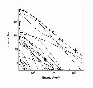
You can plot the results of the fit by executing the plot command. The results are shown below:

>>> like.plot()

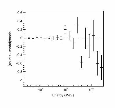The output of the plot function of the like1 UnbinnedAnalysis object shows:

• Left: the contribution of each of the objects in the model to the total model, and plots the data points on top.
• Right: the residuals of the likelihood fit to the data.Notice that the fit is poor in the second to last bin.

Now, check if NewMinuit converged.

>>> print likeobj.getRetCode()
156


If you get anything other than '0' here, than NewMinuit didn't converge. There are several reasons that we might not get convergance:

• The culprit is usually a parameter (or parameters) in the model that reach the limits set in the XML file. If this happens the minimizer cannot reach the formal minimum, and hence cannot calculate the curvature.
• Often the problem is with spectral shape parameters (PL index etc..), so simply freezing the shape of all spectral parameters to their values from the full time period (and certainly for weaker background sources) when fitting a shorter time period may solve the problem. Remember that the 2FGL used a full 2 years of data and we're using a much shorter time period here
• Weak background sources are more likely to cause problems, so you could consider just freezing them completely (or removing them from the model). For example a background source from the catalog that is detected at TS~=25 in 2 years could cause convergence problems in a 1-month light curve, where it will often not be detectable at all.
• If there are no parameters at their limits, then increasing the overall convergence tolerance may help - try using a value of 1E-8 for the absolute tolerance.
• If that doesn't help then try to systematically simplify the model. Progressively freeze all sources, starting with those at the edge of the ROI in and moving in until you get a model simple enough for the minimizer to work reliably. For example if you are using a 10 degree ROI, you could start by freezing all background sources further than 7 degrees from the source of interest, and move to 5 degrees if that doesn't solve the problem.

Let's check the TS values of the sources in the model.

>>> sourceDetails = {}
>>> for source in like.sourceNames():
>>>    sourceDetails[source] = like.Ts(source)
>>> print sourceDetails
{'_2FGLJ1504.3+1029': 137.89010867127217,
'_2FGLJ1505.1+0324': 1.4554038851056248,
'_2FGLJ1506.6+0806': 0.6319234665716067,
'_2FGLJ1506.9+1052': 10.135194335016422,
'_2FGLJ1512.2+0201': 0.6812909973086789,
'_2FGLJ1516.9+1925': 0.9614642116939649,
'_2FGLJ1540.4+1438': 0.1662015556357801,
'_2FGLJ1543.7-0241': 0.2741807899437845,
'_2FGLJ1546.1+0820': 14.193628361565061,
'_2FGLJ1548.3+1453': 34.417974132462405,
'_2FGLJ1549.5+0237': 167.3978806141531,
'_2FGLJ1550.7+0526': 41.914737970684655,
'_2FGLJ1551.9+0855': 36.993387795984745,
'_2FGLJ1553.5+1255': 960.2233608112438,
'_2FGLJ1553.5-0324': 0.20312158192973584,
'_2FGLJ1555.7+1111': 2507.2101972175296,
'_2FGLJ1602.4+2308': 0.048021055408753455,
'_2FGLJ1607.0+1552': 167.2468241514871,
'_2FGLJ1608.5+1029': 70.93913898838218,
'_2FGLJ1612.0+1403': 14.84744038071949,
'_2FGLJ1624.4+1123': 10.374797308351845,
'_2FGLJ1625.2-0020': -0.003496127901598811,
'_2FGLJ1641.0+1141': 0.5737337245373055,
'_2FGLJ1650.8+0830': 0.7823014587629586,
'gll_iem_v05_rev1': 4341.037063298281,
'iso_source_v05': 1481.2477740809554}


There's a source with a TS value less than 0 (2FGLJ1625.2-0020). This should never happen unless the minimization failed (which it did in this case). Let's remove that source and try fitting again and check the return code again.

>>> like.deleteSource('_2FGLJ1625.2-0020')
>>> like.fit(verbosity=0,covar=True,optObject=likeobj)
444127.27861489786
>>> print likeobj.getRetCode()
156


Well, this is frustrating. Let's look at the TS values now.

>>> sourceDetails = {}
>>> for source in like.sourceNames():
>>>    sourceDetails[source] = like.Ts(source)
>>> print sourceDetails
{'_2FGLJ1504.3+1029': 137.8713692999445,
'_2FGLJ1505.1+0324': 1.4546070069773123,
'_2FGLJ1506.6+0806': 0.6316319842590019,
'_2FGLJ1506.9+1052': 10.132809510920197,
'_2FGLJ1512.2+0201': 0.6807532904203981,
'_2FGLJ1516.9+1925': 0.9605303853750229,
'_2FGLJ1540.4+1438': 0.16500923444982618,
'_2FGLJ1543.7-0241': 0.2740611215122044,
'_2FGLJ1546.1+0820': 14.191890330519527,
'_2FGLJ1548.3+1453': 34.412785098771565,
'_2FGLJ1549.5+0237': 167.39689852984156,
'_2FGLJ1550.7+0526': 41.9100884340005,
'_2FGLJ1551.9+0855': 36.99264199298341,
'_2FGLJ1553.5+1255': 960.2332838408183,
'_2FGLJ1553.5-0324': 0.20308500924147666,
'_2FGLJ1555.7+1111': 2507.1926636261633,
'_2FGLJ1602.4+2308': 0.04746619611978531,
'_2FGLJ1607.0+1552': 167.24322002776898,
'_2FGLJ1608.5+1029': 70.93541790707968,
'_2FGLJ1612.0+1403': 14.837796344421804,
'_2FGLJ1624.4+1123': 10.371575461700559,
'_2FGLJ1641.0+1141': 0.5731006258865818,
'_2FGLJ1650.8+0830': 0.7816251839976758,
'gll_iem_v05_rev1': 4341.3350996187655,
'iso_source_v05': 1481.1248766540084}


Ok, we're going to do something drastic here and really simplify the model by removing sources with TS levels below 9 (about 3 sigma). This should help. This process is usually the most frustrating part of any analysis and could take some work to get convergence. In the end, go back up to the recipe above to get things to work. It's very important that you do so. If your fit doesn't converge then you cannot trust your results.

>>> for source,TS in sourceDetails.iteritems():
>>>    print source, TS
>>>    if (TS < 9.0):
>>>       print "Deleting..."
>>>       like.deleteSource(source)
_2FGLJ1540.4+1438 0.16500923445
Deleting...
_2FGLJ1555.7+1111 2507.19266363
_2FGLJ1543.7-0241 0.274061121512
Deleting...
_2FGLJ1505.1+0324 1.45460700698
Deleting...
_2FGLJ1506.6+0806 0.631631984259
Deleting...
_2FGLJ1551.9+0855 36.992641993
_2FGLJ1608.5+1029 70.9354179071
_2FGLJ1550.7+0526 41.910088434
_2FGLJ1512.2+0201 0.68075329042
Deleting...
_2FGLJ1553.5-0324 0.203085009241
Deleting...
_2FGLJ1607.0+1552 167.243220028
_2FGLJ1553.5+1255 960.233283841
_2FGLJ1602.4+2308 0.0474661961198
Deleting...
_2FGLJ1504.3+1029 137.8713693
_2FGLJ1516.9+1925 0.960530385375
Deleting...
_2FGLJ1548.3+1453 34.4127850988
_2FGLJ1641.0+1141 0.573100625887
Deleting...
_2FGLJ1549.5+0237 167.39689853
_2FGLJ1546.1+0820 14.1918903305
gll_iem_v05_rev1 4341.33509962
_2FGLJ1506.9+1052 10.1328095109
_2FGLJ1650.8+0830 0.781625183998
Deleting...
_2FGLJ1612.0+1403 14.8377963444
_2FGLJ1624.4+1123 10.3715754617
iso_source_v05 1481.12487665
>>> like.fit(verbosity=0,covar=True,optObject=likeobj)
444130.1463973735
>>> print likeobj.getRetCode()
0


Excellent. We have convergence and can move forward. Note, however, that this doesn't mean you have the 'right' answer. It just means that you have the answer assuming the model you put in. This is a subtle feature of the likelihood method.

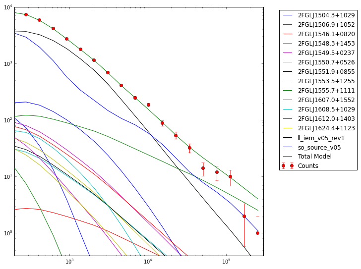
Let's take a look at the residuals and overal model using matplotlib.

>>> import matplotlib.pyplot as plt
>>> import numpy as np
We need to import these two modules for plotting and some other stuff. They are included in the Science Tools. >>> E = (like.energies[:-1] + like.energies[1:])/2.
The 'energies' array are the endpoints so we take the midpoint of the bins.
>>> plt.figure(figsize=(9,9))
>>> plt.ylim((0.4,1e4))
>>> plt.xlim((200,300000))
>>> sum_model = np.zeros_like(like._srcCnts(like.sourceNames()[0]))
>>> for sourceName in like.sourceNames():
>>>    sum_model = sum_model + like._srcCnts(sourceName)
>>>    plt.loglog(E,like._srcCnts(sourceName),label=sourceName[1:])
>>> plt.loglog(E,sum_model,label='Total Model')
>>> plt.errorbar(E,like._Nobs(),yerr=np.sqrt(like._Nobs()), fmt='o',label='Counts')
>>> plt.legend(bbox_to_anchor=(1.05, 1), loc=2)
>>> plt.show()
>>> resid = (like._Nobs() - sum_counts)/sum_counts
>>> resid_err = (np.sqrt(like._Nobs())/sum_counts)
>>> plt.figure(figsize=(9,9))
>>> plt.xscale('log')
>>> plt.errorbar(E,resid,yerr=resid_err,fmt='o')
>>> plt.axhline(0.0,ls=':')
>>> plt.show()


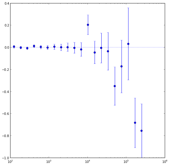
These are just some examples of how to access the underlying data from the python tools. As you can see, most of the information is accessable if you dig around. Note that the residuals aren't that great in several bins, especially at high energies. This could be a missing source or that we're not modelling a bright source very well. If you look up at the model plot, the high energy tail of PG1553 might be biasing the fit high at high energies and we might get a better fit with a log-parabola or broken power-law. That's for another day though.

Let's check out the final parameters of the fit for PG1553.

>>> like.model['_2FGLJ1555.7+1111']
_2FGLJ1555.7+1111
Spectrum: PowerLaw
26 Prefactor: 3.002e+00 1.422e-01 1.000e-04 1.000e+04 ( 1.000e-12)
27 Index: 1.629e+00 3.174e-02 0.000e+00 5.000e+00 (-1.000e+00)
28 Scale: 2.239e+03 0.000e+00 3.000e+01 5.000e+05 ( 1.000e+00) fixed
>>> like.flux('_2FGLJ1555.7+1111',emin=200)
4.835353419305393e-08
>>> like.fluxError('_2FGLJ1555.7+1111',emin=200)
2.7965147029905621e-09


This is pretty close to the paper's results (index of 1.63 +- 0.03 vs 1.68 +- 0.03 and an integral flux above 200 MeV of 4.8 +- 0.3 vs 5.0 +- 0.3). This is very good considering we are using a different model, different diffuse models and a different dataset than was used in the paper.

You can also get the TS value for a specific source:

>>> like.Ts('_2FGLJ1555.7+1111')
2505.197927852627


you can calculate how many standard deviations (σ) this corresponds to. (Remember that the TS value is ∼ σ².)

>>> np.sqrt(like.Ts('_2FGLJ1555.7+1111'))
50.051952288123857


Let's save the results.

>>> like.logLike.writeXml('PG1553_fit.xml')

Create some TS Maps

If you want to check on your fit you should probably make a test statistic (TS) map of your region at this point. This will allow you to check and make sure that you didn't miss anything in the ROI (like a source not in the catalog you used). A TS map is created by moving a putative point source through a grid of locations on the sky and maximizing the log(likelihood) at each grid point. We're going to make two TS Maps. If you have access to multiple CPUs, you might want to start one of the maps running in one terminal and the other in another one since this will take several hours to complete. Our main goal is to create one TS Map with PG1553 included in the fit and another without. The first one will allow us to make sure we didn't miss any sources in our ROI and the other will allow us to see the source. All of the other sources in our model file will be included in the fit and shouldn't show up in the final map.

If you don't want to create these maps, go ahead and skip the following steps and jump to the section on making a butterfly plot. The creation of these maps is optional and is only for double checking your work. You should still modify your model fit file as detailed in the following paragraph.

First open a new terminal and then copy PG1553_fit.xml as PG1553_fit_TSMap.xml. Modify PG1553_fit_TSMap.xml to make everything fixed by changing all of the free="1" statements to free="0". Modify the lines that look like:

to look like:

Then copy it and call it PG1553_fit_noPG1553.xml and comment out (or delete) the PG1553 source. If you want to generate the TS maps, in one window do the following:

>>> my_apps.TsMap['statistic'] = "UNBINNED"
>>> my_apps.TsMap['scfile'] = "PG1553_SC.fits"
>>> my_apps.TsMap['evfile'] = "PG1553_filtered_gti.fits"
>>> my_apps.TsMap['expmap'] = "PG1553_expMap.fits"
>>> my_apps.TsMap['expcube'] = "PG1553_ltCube.fits"
>>> my_apps.TsMap['srcmdl'] = "PG1553_fit_TSMap.xml"
>>> my_apps.TsMap['irfs'] = "CALDB"
>>> my_apps.TsMap['optimizer'] = "NEWMINUIT"
>>> my_apps.TsMap['outfile'] = "PG1553_TSmap_resid.fits"
>>> my_apps.TsMap['nxpix'] = 25
>>> my_apps.TsMap['nypix'] = 25
>>> my_apps.TsMap['binsz'] = 0.5
>>> my_apps.TsMap['coordsys'] = "CEL"
>>> my_apps.TsMap['xref'] = 238.929
>>> my_apps.TsMap['yref'] = 11.1901
>>> my_apps.TsMap['proj'] = 'STG'
>>> my_apps.TsMap.run()


In another window do the following:

>>> my_apps.TsMap['statistic'] = "UNBINNED"
>>> my_apps.TsMap['scfile'] = "PG1553_SC.fits"
>>> my_apps.TsMap['evfile'] = "PG1553_filtered_gti.fits"
>>> my_apps.TsMap['expmap'] = "PG1553_expMap.fits"
>>> my_apps.TsMap['expcube'] = "PG1553_ltCube.fits"
>>> my_apps.TsMap['srcmdl'] = "PG1553_fit_noPG1553.xml"
>>> my_apps.TsMap['irfs'] = "CALDB"
>>> my_apps.TsMap['optimizer'] = "NEWMINUIT"
>>> my_apps.TsMap['outfile'] = "PG1553_TSmap_noPG1553.fits"
>>> my_apps.TsMap['nxpix'] = 25
>>> my_apps.TsMap['nypix'] = 25
>>> my_apps.TsMap['binsz'] = 0.5
>>> my_apps.TsMap['coordsys'] = "CEL"
>>> my_apps.TsMap['xref'] = 238.929
>>> my_apps.TsMap['yref'] = 11.1901
>>> my_apps.TsMap['proj'] = 'STG'
>>> my_apps.TsMap.run()


This will take a while (over 3 hours each) so go get a cup of coffee. The final TS maps will be pretty rough since we selected to only do 25x25 0.5 degree bins but it will allow us to check if anything is missing and go back and fix it. These rough plots aren't publication ready but they'll do in a pinch to verify that we've got the model right.

Once the TS maps have been generated, open them up in whatever viewing program you wish. Here's how you could use Matplotlib to do it.

>>> import pyfits
>>> residHDU = pyfits.open('PG1553_TSmap_resid.fits')
>>> sourceHDU = pyfits.open('PG1553_TSmap_noPG1553.fits')
>>> fig = plt.figure(figsize=(16,8))
>>> plt.subplot(1,2,1)
>>> plt.imshow(residHDU[0].data)
>>> plt.colorbar()
>>> plt.subplot(1,2,2)
>>> plt.imshow(sourceHDU[0].data)
>>> plt.colorbar()
>>> plt.show()


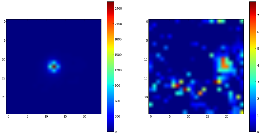
You can see that the 'noPG1553' map (left) has a prominent source in the middle of the ROI. This is PG 1553+113 and if you execute the following you can see that the TS value of the maxiumum pretty well with the TS value of PG 1553+113 that we arrived at above.

>>> np.max(sourceHDU[0].data)
2523.687

If you then look at the 'residuals' plot (right), you can see that it's pretty flat in TS space (the brightest pixel has a TS value of around 8).

>>> np.max(residHDU[0].data)
7.8157892

This indicates that we didn't miss any significant sources. If you did see something significant (TS > 20 or so), you probably should go back and figure out what source you missed.

Produce the Butterfly Plot

Now we'll produce the butterfly plot. First, get the differential flux, the decorrelation (pivot) energy, and the index. You'll also need the errors.

>>> N0 = like.model['_2FGLJ1555.7+1111'].funcs['Spectrum'].getParam('Prefactor').value()
>>> N0_err = like.model['_2FGLJ1555.7+1111'].funcs['Spectrum'].getParam('Prefactor').error()
>>> I = like.model['_2FGLJ1555.7+1111'].funcs['Spectrum'].getParam('Index').value()
>>> I_err = like.model['_2FGLJ1555.7+1111'].funcs['Spectrum'].getParam('Index').error()
>>> E0 = like.model['_2FGLJ1555.7+1111'].funcs['Spectrum'].getParam('Scale').value()


Calculate the Butterfly Plot

We need to calculate the differential flux at several energy points as well as the error on that differential flux. The differential flux is defined as:

and the error on that flux is defined as:

Where cov_γγ = σ_γ² where γ is the spectral index.

So, let calculate F(E) and F(E) +/- Δ F(E) so that we can plot it. First, define a function for the flux and one for the error on the flux.

>>> f = lambda E,N0,E0,gamma: N0*(E/E0)**(-1*gamma)
>>> ferr = lambda E,F,N0,N0err,E0,cov_gg: F*np.sqrt(N0err**2/N0**2 + ((np.log(E/E0))**2)*cov_gg)


Now, generate some energies to evaluate the functions above and evaluate them.

>>> E = np.logspace(2,5,100)
>>> F = f(E,N0,E0,gamma)
>>> Ferr = ferr(E,F,N0,N0_err,E0,cov_gg)


Now you can plot this. Here we're multiplying the flux by E² for clarity.

>>> plt.figure(figsize=(8,8))
>>> plt.xlabel('Energy [MeV]')
>>> plt.ylabel(r'E$^2$ dN/dE [MeV s$^{-1}$ cm$^{-2}$]')
>>> plt.loglog(E,E**2*(F+Ferr))
>>> plt.loglog(E,E**2*(F-Ferr))
>>> plt.plot(E,E**2*F)
>>> plt.show()


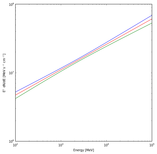
The red line is the nominal fit and the blue and green lines are the 1 sigma contours.

Generate Spectral Points

To generate spectral points to plot on top of the butterfly that we just produced, you need to go back to the data selection part and use gtselect (filter in python) to divide up your data set in energy bins and run the likelihood fit on each of these individual bins. Luckily, there's a script that does this for us that we'll employ to get a final result. This script also generates the butterfly plot we just produced so you won't have to redo that again and it also does a lot of checks on the data to make sure that everything is going ok. If you've made it this far, you might be a little curious as to why we didn't jump right into using this tool but now you're in a position to play with the python tools and make them do what you want them to. The script is also much more careful in handling units and saving everything to files than we have been in this interactive session.

So download the likeSED.py user contributed tool (it's in the SED_scripts package) and load it up into python. You can find information on the usage of this tool on the same page where you downloaded it. It can be used to generate an SED plot for both binned and unbinned analyses but we're only going to work on a binned analysis here.

>>> from likeSED import *
This is likeSED version 12.1, modified to handle Pass 7 selections.


Now you need to create a likeInput object that takes our unbinnedAnalysis object, the source name and the number of bins we want as arguments. We're going to make 9 bins here like in the paper and we're also going to make custom bins and bin centers. You can have the module chose bins and bin centers for you (via the getECent function) but we're going to do it this way so we can have the double-wide bin at the end. We're also going to use the 'fit2' file (the result of our fit on the full dataset with the NewMinuit optimizer) for the fits of the individual bins but we need to edit it first to make everything fixed except for the integral value of PG 1553+113. Go ahead and do that now. We're basically assuming that the spectral index is the same for all bins and that the contributions of the other sources within the ROI are not changing with energy.

>>> inputs = likeInput(like,'_2FGLJ1555.7+1111',nbins=9)
>>> inputs.plotBins()


This last step will take a while (approximately 30 minutes) because it's creating an expmap and event file for each of the bins that we requested (look in your working directory for these files). Once it is done we'll tell it to do the fit of the full energy band and make sure we request that it keep the covariance matrix. Then we'll create a likeSED object from our inputs, tell it where we want our centers to be and then fit each of the bands. After this is done, we can plot it all with the Plot function.

>>> inputs.fullFit(CoVar=True)
Full energy range model for _2FGLJ1555.7+1111:
_2FGLJ1555.7+1111
Spectrum: PowerLaw2
47 Integral: 5.111e-01 3.058e-02 1.000e-04 1.000e+04 ( 1.000e-07)
48 Index: 1.655e+00 3.302e-02 0.000e+00 5.000e+00 (-1.000e+00)
49 LowerLimit: 2.000e+02 0.000e+00 3.000e+01 5.000e+05 ( 1.000e+00) fixed
50 UpperLimit: 3.000e+05 0.000e+00 3.000e+01 5.000e+05 ( 1.000e+00) fixed

Flux 0.2-300.0 GeV 5.1e-08 +/- 3.1e-09 cm^-2 s^-1
Test Statistic 2286.90915683
>>> sed = likeSED(inputs)
>>> sed.getECent()
>>> sed.fitBands()
-Running Likelihood for band0-
-Running Likelihood for band1-
-Running Likelihood for band2-
-Running Likelihood for band3-
-Running Likelihood for band4-
-Running Likelihood for band5-
-Running Likelihood for band6-
-Running Likelihood for band7-
-Running Likelihood for band8-
>>> sed.Plot()

This produces the following three plots: a TS plot, a counts spectrum, and a butterfly plot (statistical errors only):

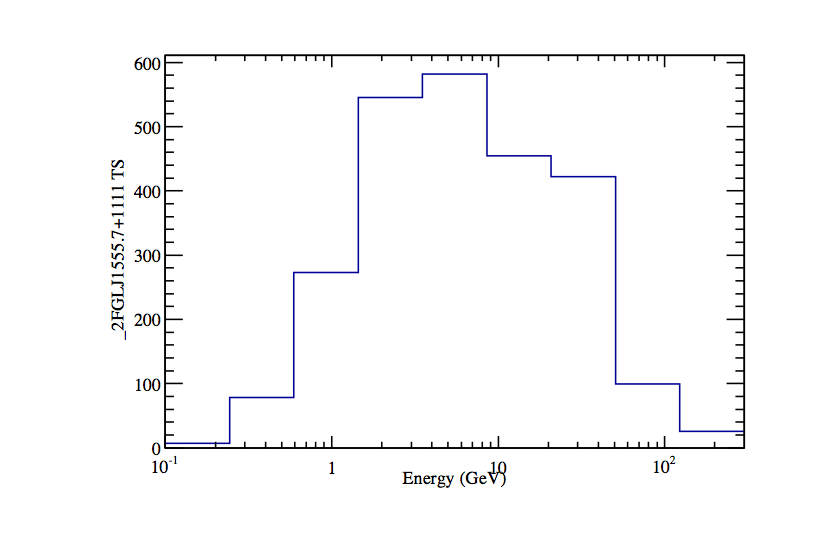
The TS plot shows the TS value for each bin in the spectrum produced by likeSED. Notice that the last bin is double-wide.

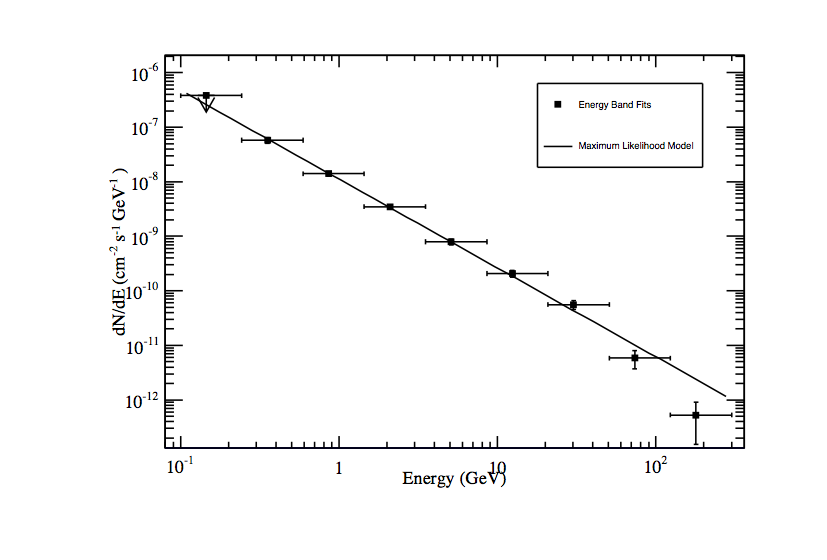
Counts spectrum produced by likeSED along with the spectral points.

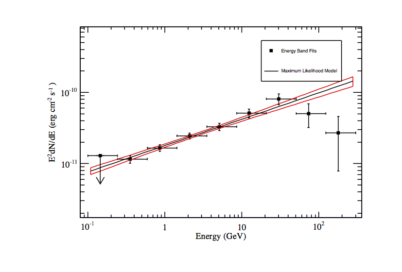
Butterfly plot along with the spectral points produced by likeSED. Note that this plot does not include the systematic errors.

Mmm, looking at that spectrum, there might be some curvature there like was hinted at in the model plot above. The butterfly model is the likelihood output and will only tell us the best fit power law since that is what we had in our model. The SED points are fits with a power-law in individual energy bands and can show us if the model we're assuming is a good assumption. Testing for curvature is for another day...

Now we're going to leave python and look at the files that likeSED produced. Open a new terminal. In your working directory you will find a bunch of _2FGLJ1555.7+1111_9bins files. These are just the event and exposure maps for each bin we selected. If you wanted to completely redo the likeSED analysis you should delete these. Some other files to note are _2FGLJ1555.7+1111_9bins_likeSEDout.fits which contains all of the data needed to reproduce the plots seen when we ran the Plot function. There is also a root file (_2FGLJ1555.7+1111_9bins_histos.root) with dumps of the plots and eps files of all of the plots. Now that we've generated a butterfly SED and individual SED data points we can move on to working on a light curve.

Building a Light Curve

The process for producing a light curve is pretty simple. We take the model fit we have (the PG1553_fit.xml file) and set all parameters to fixed except the index and integral of PG 1553+113, generate an event file for a single time bin, run gtmktime, generate an exposure cube and exposure map for that time bin and run the likelihood on that and get out the integral and index for that bin. So make a copy of the full fit model file and edit that as described above.

[user@localhost]$ cp PG1553_fit.xml PG1553_lightcurve.xml


In the paper, they did this for 2-day bins but we'll make weekly 7 day bins here just to make our job a bit easier and faster. You could also generate a light curve via Aperture Photometry which is much quicker but less rigorous. There is also a perl script in the user contributed tools that will generate lightcurves which you could use here. If you want to be more rigorous check out the LATAnalysisScripts or Enrico.

Here's a python module that should do what we want it to do: LightCurve.py. Note that this module is not completely rigorous and not suited to generate scientific results but it'll get us going in the right direction.Open the file up in your favorite text editor and have a look at what we're going to do. This file defines a simple class with two functions. One that generates all of the needed files and the other that runs a likelihood anlaysis on those files.

>>> from LightCurve import LightCurve
>>> lc = LightCurve()
>>> lc.generate_files()
**Working on range (239557417.000000,240162217.000000)**
***Running gtselect***
time -p ~/ScienceTools/x86_64-unknown-linux-gnu-libc2.12/bin/gtselect infile=PG1553_filtered.fits outfile=LC_filtered_bin0.fits ra=238.929 dec=11.1901 rad=10.0 tmin=239557417.0 tmax=240162217.0 emin=200.0 emax=200000.0 zmax=105.0 evclsmin="INDEF" evclsmax="INDEF" evclass=2 convtype=-1 phasemin=0.0 phasemax=1.0 evtable="EVENTS" chatter=2 clobber=yes debug=no gui=no mode="ql"
Done.
real 3.17
user 0.20
sys 0.08
***Running gtmktime***
time -p ~/ScienceTools/x86_64-unknown-linux-gnu-libc2.12/bin/gtmktime scfile=SC.fits sctable="SC_DATA" filter="(DATA_QUAL>0)&&(LAT_CONFIG==1)" roicut=yes evfile=LC_filtered_bin0.fits evtable="EVENTS" outfile="LC_filtered_gti_bin0.fits" apply_filter=yes overwrite=no header_obstimes=yes tstart=0.0 tstop=0.0 gtifile="default" chatter=2 clobber=yes debug=no gui=no mode="ql"
real 0.79
user 0.33
sys 0.08
***Running gtltcube***
time -p ~/ScienceTools/x86_64-unknown-linux-gnu-libc2.12/bin/gtltcube evfile="LC_filtered_gti_bin0.fits" evtable="EVENTS" scfile=PG1553_SC.fits sctable="SC_DATA" outfile=LC_expCube_bin0.fits dcostheta=0.025 binsz=1.0 phibins=0 tmin=0.0 tmax=0.0 file_version="1" zmax=180.0 chatter=2 clobber=yes debug=no gui=no mode="ql"
Working on file PG1553_SC.fits
.....................!
real 57.41
user 54.19
sys 0.70
***Running gtexpmap***
time -p ~/ScienceTools/x86_64-unknown-linux-gnu-libc2.12/bin/gtexpmap evfile=LC_filtered_gti_bin0.fits evtable="EVENTS" scfile=PG1553_SC.fits sctable="SC_DATA" expcube=LC_expCube_bin0.fits outfile=LC_expMap_bin0.fits irfs="CALDB" srcrad=20.0 nlong=120 nlat=120 nenergies=20 submap=no nlongmin=0 nlongmax=0 nlatmin=0 nlatmax=0 chatter=2 clobber=yes debug=no gui=no mode="ql"
The exposure maps generated by this tool are meant
to be used for *unbinned* likelihood analysis only.
Do not use them for binned analyses.
Computing the ExposureMap using LC_expCube_bin0.fits
....................!
real 88.86
user 85.68
sys 0.67

...The output from the calculations of the other bins will be here...


Now run the likelihood analysis on each bin.

>>> lc.runLikelihood()
**Working on range (239557417.000000,240162217.000000)
***Running likelihood analysis***
**Working on range (240162217.000000,240767017.000000)
***Running likelihood analysis***
**Working on range (240767017.000000,241371817.000000)
***Running likelihood analysis***
**Working on range (241371817.000000,241976617.000000)
***Running likelihood analysis***
**Working on range (241976617.000000,242581417.000000)
***Running likelihood analysis***
**Working on range (242581417.000000,243186217.000000)
***Running likelihood analysis***
**Working on range (243186217.000000,243791017.000000)
***Running likelihood analysis***
**Working on range (243791017.000000,244395817.000000)
***Running likelihood analysis***
**Working on range (244395817.000000,245000617.000000)
***Running likelihood analysis***
**Working on range (245000617.000000,245605417.000000)
***Running likelihood analysis***
**Working on range (245605417.000000,246210217.000000)
***Running likelihood analysis***
**Working on range (246210217.000000,246815017.000000)
***Running likelihood analysis***
**Working on range (246815017.000000,247419817.000000)
***Running likelihood analysis***
**Working on range (247419817.000000,248024617.000000)
***Running likelihood analysis***


Now you can plot the results that are stored in public variables associated with the lc object. First import a helper module and get the MET times in a useful format.

>>> from matplotlib import dates as mdates
>>> times = mdate.epoch2num(978307200+ (lc.times[:-1]+lc.times[1:])/2.)


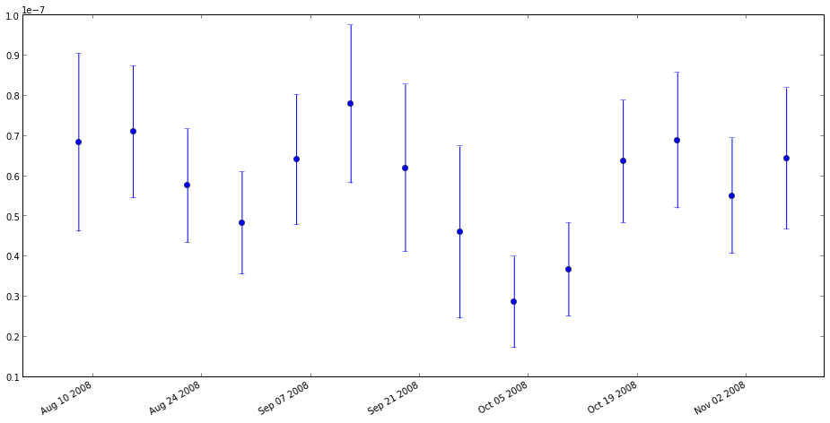
Now, plot the flux.

>>> plt.figure(figsize=(16,8))
>>> plt.xlim((mdate.datetime.date(2008,8,1),mdate.datetime.date(2008,11,12)))
>>> plt.errorbar(mdate.num2date(times),lc.IntFlux,yerr=lc.IntFluxErr,fmt='o')
>>> plt.gcf().autofmt_xdate()
>>> plt.show()


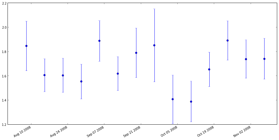
Plot the index.

>>> plt.figure(figsize=(16,8))
>>> plt.xlim((mdate.datetime.date(2008,8,1),mdate.datetime.date(2008,11,12)))
>>> plt.errorbar(mdate.num2date(times),lc.Gamma,yerr=lc.GammaErr,fmt='o')
>>> plt.gcf().autofmt_xdate()
>>> plt.show()


You should also do some checks to make sure everything is ok. Your first inspection should be to make sure that the fit converged. Remember the return code we checked from the fit above. Well, we saved that here as well (check the LightCurve module to figure out how).

>>> print lc.retCode
[ 0. 0. 0. 0. 0. 0. 0. 0. 0. 0. 0. 0. 0. 0.]


They're all zero so we're good on that front. You should also look for any abnormally large or small error bars in the lightcurves. Another thing to check is the ratio of (Flux/FluxError) vs. (Npred/sqrt(Npred). If the source model converged and predicts Npred counts than the ratio of flux error to flux should not be better than that of the Poisson counts underlying the measurement: sqrt(Npred)/Npred. It so happens that Npred has been saved as well and we can make a handy plot.

>>> plt.figure(figsize=(8,8))
>>> plt.plot(lc.IntFlux / lc.IntFluxErr, lc.npred / np.sqrt(lc.npred),'o')
>>> plt.show()

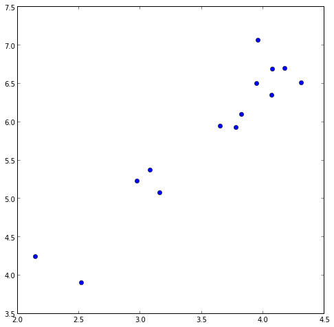
If there are any outliers, you've got issues.

Upper Limits

One thing you might want to do is to make one of the data points into an upper limit instead of an actual data point. Since we've increased the width of these bins from the paper you can see that we've got good statistics for each of the bins. Look at the TS values.

>>> print lc.TS
[ 67.65386286 152.94854511 135.67525243 108.05381208 84.26033027
175.20508563 57.79851384 29.51864172 51.30961321 127.74174233
137.71006555 94.25161777 73.06292764 104.48774638


The smallest TS values is 29.5 in bin 7 (starting with 0). Let's calculate an upper limit for that bin.

>>> bin7obs = UnbinnedObs('LC_filtered_gti_bin7.fits', 'PG1553_SC.fits', expMap='LC_expMap_bin7.fits', expCube='LC_expCube_bin7.fits', irfs='CALDB')
>>> bin7like = UnbinnedAnalysis(bin7obs,'PG1553_lightcurve.xml',optimizer='NewMinuit')
>>> bin7like.fit(verbosity=0,covar=True)
7660.540598608494
>>> bin7like.Ts('_2FGLJ1555.7+1111')
29.51864172144451
>>> from UpperLimits import UpperLimits
>>> ul=UpperLimits(bin7like)
>>> ul['_2FGLJ1555.7+1111'].compute()
0 2.22070536418 5.68526775169e-06 8.04693300166e-08
1 2.5327940203 0.0710910622147 8.84678970055e-08
2 2.84488267642 0.271933353548 9.62511455254e-08
3 3.15697133255 0.579646699965 1.03762508052e-07
4 3.46905998867 0.977183670085 1.11078673529e-07
5 3.77664993599 1.44414957542 1.1814688798e-07
(1.1679747829041963e-07, 3.7179272050740706)
>>> print ul['_2FGLJ1555.7+1111'].results
[1.17e-07 ph/cm^2/s for emin=100.0, emax=300000.0, delta(logLike)=1.35]


The results are in a python list and it keeps track of all the upper limits you've computed. Now you can use this upper limit in your light curve if you so choose. This method can also be used to calculate an upper limit on the full data set if you are analyzing a non-detectable source.

There's also a Baysian upper limit method avaialble if you would rather use that.

>>> import IntegralUpperLimit as IUL
>>> limit,results = IUL.calc_int(bin7like,'_2FGLJ1555.7+1111',cl=0.95)
>>> print limit
1.14855208655e-07


Finished

So, it looks like we've reproduced all of the results in the PG 1553+113 paper. I hope that you have a better idea of what you can do with the python tools. This tutorial should be a jumping off point into writing your own analysis scripts.

---

Last updated by: Jeremy S. Perkins 05/07/2014