This webpage is kept for archival purposes only and is no longer updated or maintained.

Fermi-Swift GRB Data Analysis Workshop

November 8-12, 2010
Goddard Space Flight Center
Greenbelt, MD

Fermi LAT

Software

Download and install the ScienceTools software from the Fermi Science Support Center:

http://fermi.gsfc.nasa.gov/ssc/data/analysis/software/

NB: Sourcing either of the setup files, fermi_init.[c]sh, for the LAT software will set the CALDB-related environment variables, thereby over-writing any existing values of those variables.

Data Download

For the workshop exercise, we will be analyzing LAT data from GRB 090510.

1. From the GCN Circular data, determine the initial burst location and trigger time. For GRB 090510, the GCN archive has the relevant circulars. Although there are several follow-up circulars from Swift and Fermi, we will extract the LAT data based on the earliest Swift circular and will derive a location and error circle based on the LAT data alone using the circular info as input. That circular is # 9331 and gives the trigger time and XRT position as

T0 = 00:23:00 UT, 10-05-2009 RA = 33.55195 (J2000) Dec = -26.58345

2. Convert the trigger time to Fermi Mission Elapsed Time using the xTime web page:

T0 = 263607782.000 MET

3. Download the desired data from the FSSC data server data query page. Although the Swift/BAT and Fermi/GBM circulars indicate that this is a short burst, we will download the LAT data as late as 5 hours after the trigger to look for possible extended/afterglow emission in the LAT data. In order to search for possible precursor emission, we will select data 15 mins before the trigger:

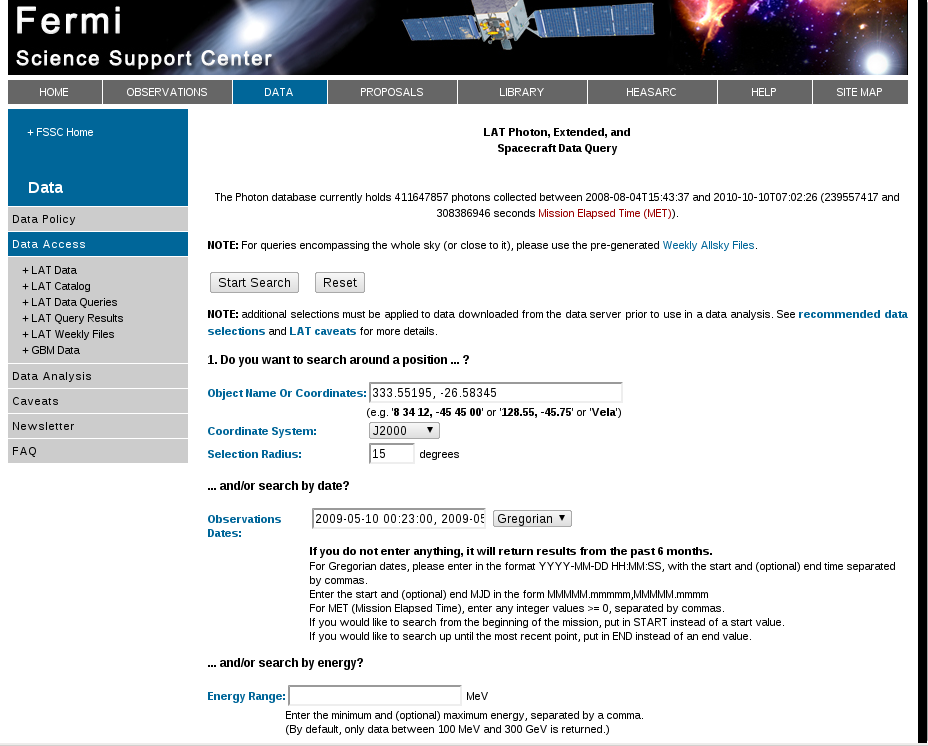
Note that one can specify the desired time range as in Gregorian format, MET or MJD format. Be sure that the "Photon Data" and "Spacecraft Data" options are selected (the default):

Data Subselection

0. Symlink the download filenames (optional)

After dowloading from the FSSC site, you should have two files with rather unwieldy names. I'll symlink these to some shorter names and will use those names hereafter:

% ls -l L*.fits
-rw-rw-r— 1 jchiang jchiang 2583360 2010-10-10 10:34 L101010133334E0D2F37E61_PH00.fits
-rw-rw-r— 1 jchiang jchiang 138240 2010-10-10 10:34 L101010133334E0D2F37E61_SC00.fits
% ln -s L101010133334E0D2F37E61_PH00.fits FT1.fits
% ln -s L101010133334E0D2F37E61_SC00.fits FT2.fits

1. Filter out Earth limb emission.

The FT1.fits file will contain all of the photon data within 15 degrees of the XRT position in the time range (263606880, 263625780) MET. Most of these events will be Earth limb emission, which arise from cosmic ray interactions with the Earth's atmosphere. Here's a plot (made using fv) of the measured zenith angle distribution of the events in the FT1 file:

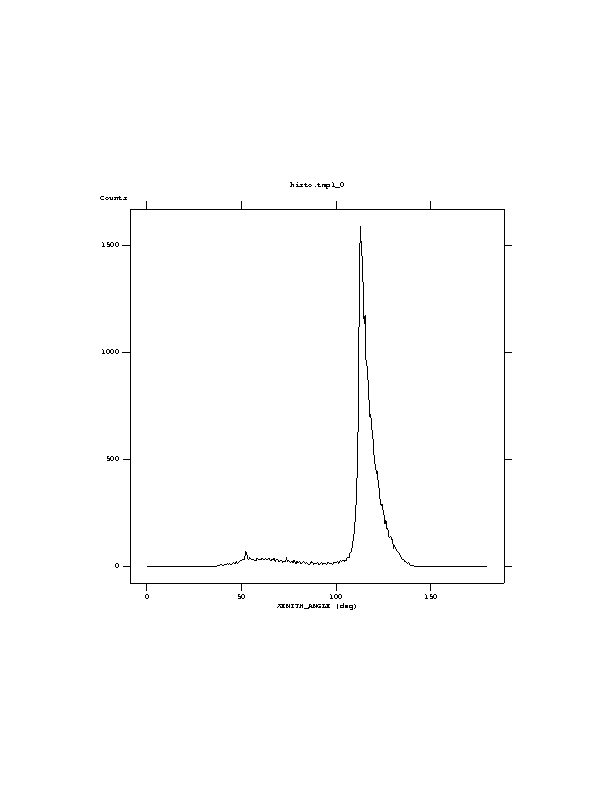
To filter these out, we will apply a zenith angle cut of 105 deg using the gtselect tool:

% gtselect evclsmin=1
Input FT1 file[] FT1.fits
Output FT1 file[] filtered_zmax105.fits
RA for new search center (degrees) (0:360) [INDEF]
Dec for new search center (degrees) (-90:90) [INDEF]
radius of new search region (degrees) (0:180) [INDEF]
start time (MET in s) (0:) [INDEF]
end time (MET in s) (0:) [INDEF]
lower energy limit (MeV) (0:) [30]
upper energy limit (MeV) (0:) [300000]
maximum zenith angle value (degrees) (0:180) [180] 105
Done.
%

Note that there is a hidden parameter, evclsmin, that sets the minimum event class selection. By default, the FSSC has set evclsmin=3 in the gtselect.par file. This corresponds to the most stringent photon selection criteria—-the so-called "diffuse" class photons. For some aspects of the GRB analysis, we will want to use the lower quality photon selection, the "transient" class events. These cuts are optimized for transient sources for which the relevent timescales are sufficiently short that the additional residual charged particle backgrounds are much less significant. To obtain transient class events, we must set evclsmin=1 at the command line.

2. Review data cuts on photon data (optional)

At this point, it might be useful to review the cuts that have been applied to the data to be sure that the desired data selections are present. The effective data selections are stored in "data sub-space" keywords in the EVENTS header of the FT1 file. The gtvcut tool can be used to display those selections:

% gtvcut
Input FITS file[] filtered_zmax105.fits
Extension name[EVENTS]
DSTYP1: POS(RA,DEC)
DSUNI1: deg
DSVAL1: CIRCLE(333.55195,-26.58345,15)

DSTYP2: TIME
DSUNI2: s
DSVAL2: TABLE
DSREF2: :GTI

GTIs:
263606880 263610581.093
263611975.93 263616663.086
263617932.93 263622730.085
263623585.931 263625780

DSTYP3: ENERGY
DSUNI3: MeV
DSVAL3: 100:300000

DSTYP4: EVENT_CLASS
DSUNI4: dimensionless
DSVAL4: 1:4

DSTYP5: ZENITH_ANGLE
DSUNI5: deg
DSVAL5: 0:105<

%

Here we see the cuts that were applied by the FSSC data server:

15 degree acceptance cone cut centered on the XRT position,
100-300000 MeV energy cut,
GTIs corresponding to the out-of-SAA times in the spacecraft file, FT2.fits,

and the cuts we have applied using gtselect:

event class: 1-4,
zenith angle < 105 degrees

Data Exploration

1. Counts maps

To get an idea of how much the zenith angle filtering cleans up the data, we'll make counts maps of the extraction region using the unfiltered (FT1.fits) and filtered (filtered_zmax105.fits) data. For this, we use the gtbin tool:

% gtbin
This is gtbin version ScienceTools-v9r17p0-fssc-20100906
Type of output file (CCUBE|CMAP|LC|PHA1|PHA2) [PHA2] cmap
Event data file name[] filtered_zmax105.fits
Output file name[] cmap_zmax105.fits
Spacecraft data file name[NONE] FT2.fits
Size of the X axis in pixels[] 120
Size of the Y axis in pixels[] 120
Image scale (in degrees/pixel)[] 0.25
Coordinate system (CEL - celestial, GAL -galactic) (CEL|GAL) [CEL]
First coordinate of image center in degrees (RA or galactic l)[] 333.55195
Second coordinate of image center in degrees (DEC or galactic b)[] -26.58345
Rotation angle of image axis, in degrees[0.]
Projection method e.g. AIT|ARC|CAR|GLS|MER|NCP|SIN|STG|TAN:[AIT] STG

% gtbin
This is gtbin version ScienceTools-v9r17p0-fssc-20100906
Type of output file (CCUBE|CMAP|LC|PHA1|PHA2) [CMAP]
Event data file name[filtered_zmax105.fits] FT1.fits
Output file name[cmap_zmax105.fits] cmap_unfiltered.fits
Spacecraft data file name[FT2.fits]
Size of the X axis in pixels[120]
Size of the Y axis in pixels[120]
Image scale (in degrees/pixel)[0.25]
Coordinate system (CEL - celestial, GAL -galactic) (CEL|GAL) [CEL]
First coordinate of image center in degrees (RA or galactic l)[333.55195]
Second coordinate of image center in degrees (DEC or galactic b)[-26.58345]
Rotation angle of image axis, in degrees[0]
Projection method e.g. AIT|ARC|CAR|GLS|MER|NCP|SIN|STG|TAN:[STG]

ds9 will allow us to display the two counts maps side-by-side:

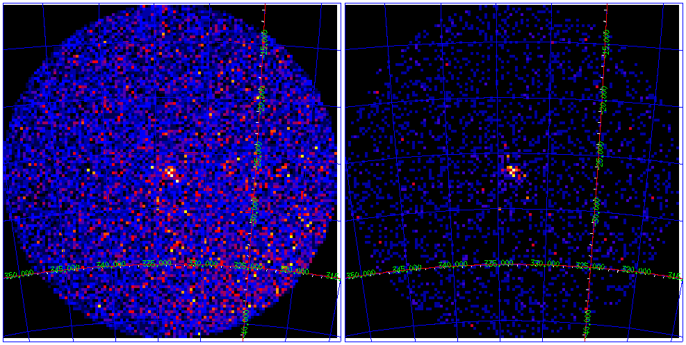
The image on the right is the data without the zmax=105 filtering and the data on the right has the filtering applied.

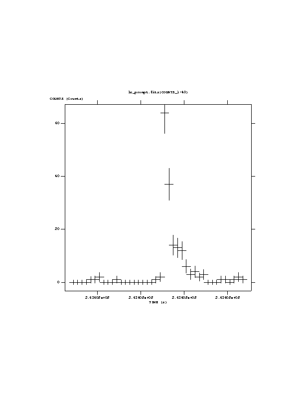
2. Light curves

gtbin can also be used to create counts light curves:

% gtbin
This is gtbin version ScienceTools-v9r17p0-fssc-20100906
Type of output file (CCUBE|CMAP|LC|PHA1|PHA2) [CMAP] lc
Event data file name[FT1.fits] filtered_zmax105.fits
Output file name[cmap_unfiltered.fits] lc_zmax105.fits
Spacecraft data file name[FT2.fits]
Algorithm for defining time bins (FILE|LIN|SNR) [LIN]
Start value for first time bin in MET[0] 263606880
Stop value for last time bin in MET[0] 263625780
Width of linearly uniform time bins in seconds[0] 100

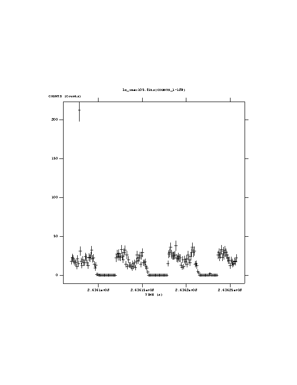
% gtbin
This is gtbin version ScienceTools-v9r17p0-fssc-20100906
Type of output file (CCUBE|CMAP|LC|PHA1|PHA2) [LC]
Event data file name[filtered_zmax105.fits]
Output file name[lc_zmax105.fits] lc_prompt.fits
Spacecraft data file name[FT2.fits]
Algorithm for defining time bins (FILE|LIN|SNR) [LIN]
Start value for first time bin in MET[263606880] 263607772
Stop value for last time bin in MET[263625780] 263607792
Width of linearly uniform time bins in seconds[100] 0.5