

GBM Gamma-Ray Burst Analysis
This section provides the information needed to obtain the GBM data and understand how the data is organized, as well as a step-by-step example of using the gtbin and gtbindef tools, the FTOOLS, and the X-Ray Spectral Fitting Package (Xspec) to analyze GBM Gamma-Ray Burst observations. Some basic familiarity with XSPEC is presumed.
Prerequisites
- If you are unfamiliar with the GBM instrument and data products, you should first review The GBM data description appended to this thread.
- gtbin, gtbindef available in the FSSC distribution of the Fermi Science Tools.
- XSPEC (see Xanadu Data Analysis for X-Ray Astronomy)
- FTOOLS available from HEASARC web site
Example: Performing a GBM Gamma-Ray Burst Analysis
First steps: use of gtbin, gtbindef, and some FTOOLS
The following is an example of how to perform a GRB analysis. The analysis was done with the GRB080730520.
- The first step in the GRB analysis is to identify the "tcat" file, and examine its contents. You may do that using the FTOOL fdump by typing:
fdump glg_tcat_all_bn080730520.fitThis will provide useful information such as which detectors triggered for this burst:
DET_MASK= '110000001100' / Triggered detectors: (0-11) - Next, run gtbin on the time-tagged event (tte) data for one of the triggered detectors to examine the burst lightcurve for that detector:
	prompt> gtbin

	Type of output file (CCUBE|CMAP|LC|PHA1|PHA2) [LC]

	Event data file name[glg_tcat_all_bn080730520.fit] glg_tte_n9_bn080730520.fit

	Output file name[glg_tcat_all_bn080730520.lc] glg_tte_n9_bn080730520.lc

	Spacecraft data file name[NONE]

	Algorithm for defining time bins (FILE|LIN|SNR) [LIN]

	Start value for first time bin in MET[INDEF]

	Stop value for last time bin in MET[INDFEF] INDEF

	Width of linearly uniform time bins in MET[0.25]
Notes:
- The choice of LC for 'Type of output file' indicates that you want to create a lightcurve.
- The choice of LIN for 'Algorithm for defining time bins' indicates that you want a linear time grid. The width of the time bins is the last parameter entered.
- The start and stop times are in Mission Elapsed Time . If you type INDEF the program takes the tstart and tstop of the original event.
- Next to plot the light curve, shifted so that the trigger time is at t=0. You may do that using the FTOOL, fcal by simply typing:
	fcalc infile=glg_tte_n9_bn080730520.lc

	outfile=glg_tte_n9_bn080730520_trig_time.lc

clname=TRIGTIME expr="Time-239113756.403240" - Finally to plot the lightcurve you may run the FTOOL fplot
fplot
infile=glg_tte_n9_bn080730520_trig_time.lc
xparm=TRIG_TIME
yparm=COUNTS
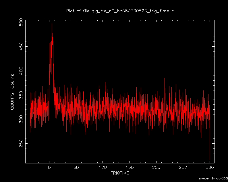
device="/Xw"The plot of the lightcurve is showed in the figure below.
Notes: We note that the fv, interactive utility, could be used as a (more powerful) alternative to fplot. For example, in fv:
- You can use the calculator function (in the 'tools' pull down menu of the 'summary' window of the extension with the quantities you want to plot) to define a new time variable equal to the time minus the trigger time. Then you can plot other variables vs. this new time variable.
- In plotting quantities vs. time you can subtract the trigger time from the time variable in the windows where the quantities to be plotted are specified.
In this case, the burst last from about 0-12 seconds. Thus, we'll use that range as a time cut in order to construct a spectrum. This is accomplished by first running gtbindef, and then rerunning gtbin in spectral (PHA2) output mode. Note that we need to shift the 0-12-s time cut back to MET by adding TRIGTIME.
Here is an example of how to run gtbindef. Before running that tool construct an ascii file, which I'll call "myTimeBinFile.txt":
239113726.403240 239113746.403240

239113756.403240 239113768.403240
The second line is the MET time rage for the burst. The first interval contains 20s of pre-burst background data, which can be used for spectral analysis. Note however, that the archive will eventually contain more accurately constructed background spectral files (see Updated files).
Next run gtbindef
gtbindef

bintype=T

binfile=myTimeBinFile.txt

outfile=myTimeBinFile.fits
Followed by gtbin, using the file you just created as input:
prompt> gtbin

Type of output file (CCUBE|CMAP|LC|PHA1|PHA2) [PHA2]

Event data file name[glg_tte_n9_bn080730520.fit]

Output file name[glg_tte_n9_bn080730520.pha]

Spacecraft data file name[NONE]

Algorithm for defining time bins (FILE|LIN|SNR) [FILE]

Name of the file containing the time bin definition[myTimeBinFile.fits]
Now this type-II pha file, along with the corresponding respons matrix file, glg_cspec_n9_bn080730520.rsp, can be analyized with XSPEC
How to run XSPEC in the analysis of the GBM data
Note: This represents the simplest example of fitting a spectrum with XSPEC. A working knowledge of the XSPEC package is assumed here. For additional information, refer to the XSPEC manual.
Start XSPEC by typing 'XSPEC' at the prompt.
XSPEC version: 12.4.0aj_d

Build Date/Time: Thu Jul 31 18:57:19 2008
Load in the PHA2 file created by gtbin:
XSPEC12>data glg_tte_n9_bn080730520.pha{2}

Spectral Data File: glg_tte_n9_bn080730520.pha{2}  Spectrum 1

Net count rate (cts/s) for Spectrum:1  1.643e+03 +/- 1.173e+01

Assigned to Data Group 1 and Plot Group 1

Noticed Channels:  1-128

Telescope: GLAST

Instrument: GBM

Channel Type: PHA

Exposure Time: 11.95 sec

No response loaded.

***Warning!  One or more spectra are missing responses,

and are not suitable for fit.
Note: Ignore the XSPEC warning that there are no associated files.
Load in the response matrix:
XSPEC12>resp glg_cspec_n9_bn080730520.rsp

Response successfully loaded.
Load in the background:
XSPEC12>back glg_tte_n9_bn080730520.pha{1}

Net count rate (cts/s) for Spectrum:1  3.682e+02 +/- 1.419e+01 (22.4 % total)
Once again, we note that optimal background spectra will be provided eventually. If available those files should be substituted here.
Ignore the lowest and highest energy channels (see GBM Data Channels to be fit).
XSPEC12>ign 1-5,100-**

5 channels (1,5) ignored in spectrum #     1

29 channels (100,128) ignored in spectrum #     1
Load a model:
XSPEC12>mo grb

5 channels (1,5) ignored in spectrum #     1

29 channels (100,128) ignored in spectrum #     1

Input parameter value, delta, min, bot, top, and max values for ...

-1       0.01        -10         -3          2          5

1:grbm:alpha>  -2       0.01        -10         -5          2         10

2:grbm:beta>  300         10         10         50       1000      10000

3:grbm:tem>     1       0.01          0          0      1e+24      1e+24

4:grbm:norm>

========================================================================

Model grbm <1> Source No.: 1   Active/On

Model Model Component  Parameter  Unit     Value

par  comp

1    1   grbm       alpha               -1.00000     +/-  0.0

2    1   grbm       beta                -2.00000     +/-  0.0

3    1   grbm       tem        keV      300.000      +/-  0.0

4    1   grbm       norm                1.00000      +/-  0.0

________________________________________________________________________

Chi-Squared =   4.420590e+06 using 94 PHA bins.

Reduced chi-squared =       49117.66 for     90 degrees of freedom

Null hypothesis probability =   0.000000e+00

Current data and model not fit yet.
Fit the data:
XSPEC12>fit 1000

Chi-Squared  Lvl Par #         1             2             3             4

93.1784      -1    -1.05918      -2.80717      248.084       0.0135866

91.0844      -1    -1.01679      -4.26303      214.978       0.0145607

89.76        -1    -0.979862     -8.85313      194.596       0.0155139

89.7599      3     -0.979862     -8.51717      194.596       0.0155139

==================================================

Variances and Principal Axes

1         2         3         4

3.33E-07 |   -0.01      0.00      0.00      1.00

2.35E-03 |    1.00      0.00      0.00      0.01

3.15E+03 |   -0.00      0.00      1.00     -0.00

4.24E+10 |    0.00      1.00     -0.00      0.00

--------------------------------------------------

================================================

Covariance Matrix

1           2           3           4

2.800e-02   2.320e+04   -1.581e+01  7.088e-04

2.320e+04   4.241e+10   -1.721e+07  6.793e+02

-1.581e+01  -1.721e+07  1.014e+04   -4.348e-01

7.088e-04   6.793e+02   -4.348e-01  1.934e-05

------------------------------------------------

========================================================================

Model grbm<1> Source No.: 1   Active/On

Model Model Component  Parameter  Unit     Value

par  comp

1    1   grbm       alpha               -0.979862    +/-  0.167326

2    1   grbm       beta                -8.51717     +/-  2.05944E+05

3    1   grbm       tem        keV      194.596      +/-  100.681

4    1   grbm       norm                1.55139E-02  +/-  4.39736E-03

________________________________________________________________________


Chi-Squared =          89.76 using 94 PHA bins.

Reduced chi-squared =         0.9973 for     90 degrees of freedom

Null hypothesis probability =   4.873082e-01
You now have to define the graphics interface before plotting the results of fitting the spectrum:
XSPEC12>cpd /Xw

XSPEC12>plot data res


XSPEC12>setplot energy

XSPEC12>plot uf
Notes:
- The XSPEC analysis can be easily generalized to handle multiple GBM detectors, using the data grouping capabiliy of XSPEC.
- The cpd command defines the graphics device, here xwindows.
- The setplot command changes the x axis from channels to energy.
- The plot command indicates that the data and model should be plotted.
The figure below shows the spectra obtained for this example.

As noted, improved background spectrum files will be provided in the future, and the instrumental response is expected to improve in accuracy as well.
The GBM data.
- Where is the GBM data?
GBM data can be obtained using HEASARC BROWSE. (See Browse Interface for GBM Tables help page.)
- The Multiplicity of the GBM files
Each burst results in a large number of files. The GBM data and the file name conventions are described in Cicerone. (See Data - GBM Data Products.)
- Channels to be fit
Most binned spectra have high and low energy channels that are beyond the instrument response function's believable energy range, are affected by non-linearities, or are overflow channels (all counts above a certain energy end up in that channel). These channels should not be included in fitting spectra; in XSPEC terminology these channels are 'ignored.' Assuming that the GBM channels run from 0 to 127 the following channels should always be ignored:
- NaI spectra—all channels below 8 keV, and then channel 127. Note that 8 keV corresponds to different channels in different NaI detectors, and therefore the low energy channels that should be ignored will vary from detector to detector.
- BGO spectra—channels 0 and 127
These are aggressive ranges (i.e., ignoring as few channels as possible) and more realistically it will be necesary to ignore a few additional channels on either end. If you find that the residual (fit minus actual count numbers) for a few channels at either end of the fitted spectrum are particularly large, then these channels are probably affected by systematics and should be ignored.
- Updated Files
The GBM team will update files as better data become available. Thus response files (files with names such as 'glg_cspec_n0_bn080808123_v00.rsp') may be updated as better burst positions become available (e.g., because Swift or the IPN provide a more accurate position that the GBM position). Background spectra (in files with names such as 'glg_cspec_n0_bn080808123_v00.bak') also require non-automated processing, and will be not appear immediatelly in the archive. A typical delay of 1-2 days is anticipated.
- Detectors to be Fit
The GBM burst data include files for all detectors, whether or not they were oriented to accumulate many counts from a burst. The NaI detectors that triggered should have accumulated the most burst counts, although if FERMI slews to point towards a long burst, other detectors will record significant burst flux.
The triggered NaI detectors will be listed in the burst catalog. But they also can be determined from the burst data files. For example, look for the 'DET_MASK' keyword in the primary header of the file that begins 'glg_tridat' (see the example below). This keyword provides a string that indicates which detectors triggered: the first character is '1' if the first NaI detector—NaI #0—triggered, and '0' if it did not, etc. Therefore the string '110000001100' means that NaI detectors 0, 1, 8 and 9 triggered.
- Time
Time in the SAE and in the FERMI data files is Mission Elapsed Time (MET), the number of seconds since midnight January 1, 2001 (UTC), as is described in Cicerone. (See Data - Time in FERMI Data Analysis.) Consequently, times will be numbers with many digits such as 239113751.4. The xTime Date/Time Conversion Utility converts between FERMI's MET and other time systems.
For analyzing GBM data you need the GBM's trigger time. This will be provided in the BROWSE catalogs, but is also found in the primary header of the GBM burst data files as the keyword 'TRIGTIME'. Note that tools such as fv allow you to read headers of the different FITS extensions.
As an aside, plotting lightcurves as counts vs FERMI's natural time system (i.e., MET) usually results in an x-axis that is not very informative because of the large difference in scale between burst durations (10's of seconds) and MET. Therefore it is useful to plot lightcurves as counts vs. time relative to the trigger time.
See:
Also see:
- Data - GBM Data Products
- Browse Interface for GBM Tables
- Combined LAT and GBM Gamma-Ray Burst analysis.
Last updated by: Analia Cillis 08/12/2009