
The Point Spread Function (PSF)
The point spread function for the LAT is a function of an incident photon's energy and inclination angle, and the event class. Furthermore, the PSF is defined in terms of a scaled-angular deviation:

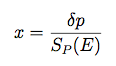
Where ![]() is the reconstructed direction and
is the reconstructed direction and ![]() is the true direction of the photon.
is the true direction of the photon.
The scale factor describes the first order variation of the PSF with energy, namely that at lower energies the PSF is dominated by multiple scattering, improves with energy, and at high energies is dominated by the spatial resolution of the LAT Silicon Tracker. If E is expressed in MeV, the scale factor is:
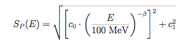
Parameters c0 and c1 are given distinct values for different event types while a common value of β is used for all event types. All of these parameters are stored in the PSF FITS file in the PSF_SCALING_PARAMS table. In Pass 8 the format of this table has been changed to include only the parameters for the given IRF event type (previously the table contained both FRONT and BACK parameters). The scaling parameters used for the P8R3_V2 IRFs are given in the table below:
| Event Type | c0 (radians) | c1 (radians) | β |
|---|---|---|---|
| FRONT | 6.38 x 10-02 | 1.26 x 10-03 | 0.8 |
| BACK | 1.23 x 10-01 | 2.22 x 10-03 | 0.8 |
| PSF0 | 1.53 x 10-01 | 5.70 x 10-03 | 0.8 |
| PSF1 | 9.64 x 10-02 | 1.78 x 10-03 | 0.8 |
| PSF2 | 7.02 x 10-02 | 1.07 x 10-03 | 0.8 |
| PSF3 | 4.97 x 10-02 | 6.13 x 10-04 | 0.8 |
| EDISP0-EDISP3 | 8.81 x 10-02 | 1.68 x 10-03 | 0.8 |
In-Flight PSF and Monte Carlo PSF
For previous data releases, the LAT team has been reporting that the Monte Carlo simulations underestimated the PSF at energies of a few GeV and above. Improvements to the Monte Carlo description of the LAT instrument introduced in Pass 8 have resolved this discrepancy. In the P8R3_V2 IRFs the PSF model is derived entirely from MC simulations and contains no in-flight correction. More details regarding the systematic uncertainties in the IRF description of the LAT PSF are given in the LAT Caveats page.
PSF Fitting Method
Once the overall energy scaling has been accounted for, additional variations in the PSF are defined for a default binning of 4 energy bins per decade, from 0.75 to 6.5 in log(Energy) (corresponding to the energy range 5.6 MeV to 3.2 TeV) and 8 bins in inclination angle (θ), equally spaced from 0.2 to 1.0 in cos(θMC). For each bin, the scaled angular deviation is calculated as described above.
The functional form of the analytical description of the LAT's Point Spread Function is derived and adapted from XMM's (a "Moffat" function, originally referred to as a "King" function in the Read et al. (2011) paper). The function is:
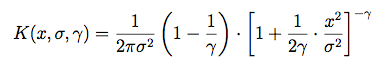
Note that this is normalized to 1 when integrated from 0 to infinity, and that the integral includes a extra factor of 2πx, because it is performed over solid angle.
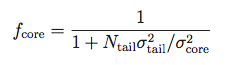
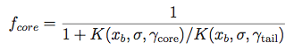
To allow for a tail in the distribution we allow for the possibilty to have two Moffat functions with different parameters:

The sigmas and gammas are stored in the PSF FITS table as SCORE,STAIL,GCORE,GTAIL. Because of the arbitrary normalization used in fitting the PSF function, fcore must be extracted from NTAIL and the other parameters. NCORE is an arbitrary overall normalization factor.
Note also that the in-flight versions of the PSF provided in the P7_V6 IRFs used a single Moffat function, so for those fcore is simply 1.
Note that the earlier P6_V3 IRFs used a slightly different scheme. In that schema the two sigma values were equal and stored as SIGMA in the FITS table. The fraction of events in the Moffat function describing the tail was fixed by matching the components at xb = sqrt(20) * σ.
Derivation of the Monte Carlo PSF
The Monte Carlo versions of the PSF are derived by first constructing a histogram of the scaled angular deviation for each bin in logarithmic Monte Carlo energy and cos(θMC). Here is an example of such a histogram for the bin centered at 7.5 GeV, and 30 degrees for front-converting events.
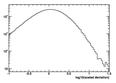
The next step of the process is to remove the extra factor of x (or r) from the solid angle integral by converting this histogram to a density histogram by dividing the contents of each bin by the bin width. In fact, a short cut is to divide by the bin center, since that is proportional to the bin width for a logarithmic scale, and the normalization is arbitrary. The resulting density histogram is then fit to extract the PSF parameters for that bin
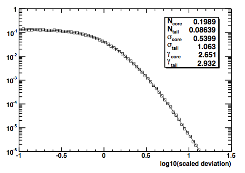
The PSF parameters for each of the bins are stored in the "RPSF" FITS table.
Fisheye Effect
The PSF parameterization used by the Fermi Fermitools assumes a functional form that is azimuthally symmetric with respect to the true direction of the incident gamma-ray. For long integration periods, azimuthal symmetry is a good approximation since a source is typically observed with a uniform distribution in azimuth angle that tends to minimize asymmetries in the average PSF distribution.
Deviations of the LAT PSF from azimuthal symmetry are caused predominantly by the fisheye effect, a selection bias in the LAT trigger and reconstruction algorithms. At low energies and high incidence angles, particles that scatter toward the LAT boresight (have a smaller apparent incidence angle) are reconstructed with higher efficiency than particles that scatter away from the LAT boresight (have a larger apparent incidence angle). This asymmetry in the reconstruction efficiency shifts the PSF distribution in the direction of the LAT boresight. This effect can be an important consideration for analyses of transient sources that are observed within a narrow range of azimuth angles and can contribute to systematic errors in both source localization and flux determination.
We characterize the bias in the LAT direction reconstruction in terms of an angular offset in a local polar coordinate system defined with respect to the true gamma-ray direction. This coordinate system is defined by the unit vectors:

where ![]() and
and ![]() are aligned with the azimuthal and polar directions with respect to the LAT boresight respectively. The angular offset between the true and reconstructed direction in local polar coordinates is then given by:
are aligned with the azimuthal and polar directions with respect to the LAT boresight respectively. The angular offset between the true and reconstructed direction in local polar coordinates is then given by:

The fisheye effect induces a negative bias in the polar direction (toward the LAT boresight). The FISHEYE_CORRECTION extension of the PSF IRF contains tables binned in true energy and incidence angle for the fisheye correction in units of scaled deviation. The correction is defined as a rotation with respect to the azimuthal axis away from the LAT boresight. The FISHEYE_CORRECTION extension contains correction tables computed with three different methods for quantifying the bias along the polar direction:
- MEAN: Mean of the distribution in polar offset angle.
- MEDIAN: Median of the distribution in polar offset angle.
- PEAK: Peak of a gaussian fit to the distribution in polar offset angle.
Although these tables are provided with the IRFs, no correction for the fisheye effect is currently supported in the Fermi Fermitools. The fisheye correction tables are intended to allow the user to quantify the systematic uncertainties that may be induced by the fisheye effect (particularly errors in the localization of transient sources that are observed at large incidence angles).
» Forward to Effective Area
» Back to the LAT IRF Overview
» Back to the beginning of the IRFs
» Back to the beginning of the Cicerone

- Curator: J.D. Myers
- NASA Official: Elizabeth Hays
- Fermi FAQ, Comments, Feedback
- › Privacy Policy and Important Notices
- › Accessibility
- › Contact NASA
- › Page Last Updated: Mon, Nov 26, 2018