
Please Note: An updated, and maintained, version of this content is available on Github as a Jupyter notebook.
Explore LAT Data (for Burst)
In this example we will examine the LAT data for a gamma-ray burst, based on the time and position derived from a GBM trigger.
You can download this tutorial as a Jupyter notebook and run it interactively. Please see the instructions for using the notebooks with the Fermitools.
Prerequisites
It is assumed that:
- You are in your working directory.
- The GBM reported a burst via
a GCN circular with the follwoing information:
- Name = GRB 080916C
- RA = 121.8
- Dec = -61.3
- Tstart = 243216766 s (Mission Elapsed Time)
- T90 = 66 s
Steps
The analysis steps are:
1. Extract the Data
Generally, one should refer to Extract LAT data tutorial, and use the time and spatial information from some source (here, a GCN notice) to make the appropiate extraction cuts from the LAT data server.
We use the following parameters to extract the data for an ROI of 20 degrees from 500s before to 1500 seconds after the trigger time:
- Search Center (RA,Dec) = (121.8,-61.3)
- Radius = 20 degrees
- Start Time (MET) = 243216266 seconds (2008-09-16T00:04:26)
- Stop Time (MET) = 243218266 seconds (2008-09-16T00:37:46)
- Minimum Energy = 30 MeV
- Maximum Energy = 300000 MeV
Note that for analyses that require the diffuse background, the standard model starts at 60 MeV.
An archive file containing the events file, spacecraft file, and associated tutorial files can be downloaded here. To extract the files, go to the directory where you saved the "LAT_explore_GRB.tgz" file and type:
prompt> tar xvfz LAT_explore_GRB.tgz
This will extract the data files used in this tutorial into the directory.
2. Data Selections
NOTE: For information on the recommended selections for burst analysis of LAT data, you should refer to the LAT Data Selection Recommendations.
To map the region of the burst, you should select a large spatial region from within a short time range bracketing the burst. For the lightcurve on the other hand, its best to select you want a small region around the burst from within a long time range. Therefore, you will need to make two different data selections. In both cases, we will use the loosest event class cut (to include all class events). This works because rapid, bright events like GRBs overwhelm the background rates for the short period of the flare.
Here we use gtselect to extract the region for the spatial mapping:
prompt>  gtselect evclass=128

Input FT1 file[] grb_events.fits

Output FT1 file[] GRB081916C_map_events.fits

RA for new search center (degrees) (0:360) [] 121.8

Dec for new search center (degrees) (-90:90) [] -61.3

radius of new search region (degrees) (0:180) [] 20

start time (MET in s) (0:) [0] 243216666

end time (MET in s) (0:) [0] 243216966

lower energy limit (MeV) (0:) [] 100

upper energy limit (MeV) (0:) [] 300000

maximum zenith angle value (degrees) (0:180) [] 180

Done.

prompt>
Notes:
- The input photon file is grb_events.fits, and the output file is GRB081916C_map_events.fits.
- We selected a circular region with radius 20 degree around the burst location (the ROI here has to fall within that selected in the data server) from a 300s time period around the trigger
- We made an additional energy cut, selecting only photons between 100 MeV and 300 GeV. This removes the low-energy, high-background events from the map.
Run gtselect again, this time with a smaller region but a longer time range. (Note that gtselect saves the values from the previous run and uses them as defaults for the next run.)
prompt>  gtselect evclass=128

Input FT1 file[grb_events.fits]

Output FT1 file[GRB090119205_map_ph.fits] GRB081916C_lc_events.fits

RA for new search center (degrees) (0:360) [121.8] 121.8

Dec for new search center (degrees) (-90:90) [-61.3] -61.3

radius of new search region (degrees) (0:180) [20] 10

start time (MET in s) (0:) [243216666] 243216266

end time (MET in s) (0:) [243216966] 243218266

lower energy limit (MeV) (0:) [100] 30

upper energy limit (MeV) (0:) [300000] 300000

maximum zenith angle value (degrees) (0:180) [180] 180

Done.

prompt>
Notes:
- A new output file, with the extension lc_events.fits has been produced.
- The search radius wss reduced to 10 degrees.
- The start to stop time range has been expanded.
- The energy range has been expanded.
3. Bin the Data
Use gtbin to bin the photon data into a map and a lightcurve.
First create the counts map:
prompt> gtbin

Type of output file (CCUBE|CMAP|LC|PHA1|PHA2) [] CMAP

Event data file name[] GRB081916C_map_events.fits

Output file name[] GRB081916C_counts_map.fits

Spacecraft data file name[NONE]

Size of the X axis in pixels[] 50

Size of the Y axis in pixels[] 50

Image scale (in degrees/pixel)[] 0.5

Coordinate system (CEL - celestial, GAL -galactic) (CEL|GAL) [] CEL

First coordinate of image center in degrees (RA or galactic l)[] 121.8

Second coordinate of image center in degrees (DEC or galactic b)[] -61.3

Rotation angle of image axis, in degrees[0.]

Projection method e.g. AIT|ARC|CAR|GLS|MER|NCP|SIN|STG|TAN:[] AIT

gtbin: WARNING: No spacecraft file: EXPOSURE keyword will be set equal to ontime.

prompt>
Notes:
- Select cmap (i.e., count map) as the output.
- When we ran gtselect we called the file from a large area GRB081916C_map_events.fits.
- The counts map file will be called GRB081916C_counts_map.fits.
- Although in gtselect we selected a circular region with a 20 degree radius, we will form a counts map with 50 pixels on a side, and 1/2 degree square pixels.
Now, we create the lightcurve. Once again, the previous inputs were saved and provided as defaults where appropriate.
prompt> gtbin

Type of output file (CCUBE|CMAP|LC|PHA1|PHA2) [CMAP] LC

Event data file name[GRB081916C_map_events.fits] GRB081916C_lc_events.fits

Output file name[GRB081916C_counts_map.fits] GRB081916C_light_curve.fits

Spacecraft data file name[NONE]

Algorithm for defining time bins (FILE|LIN|SNR) [] LIN

Start value for first time bin in MET[] 243216266

Stop value for last time bin in MET[] 243218266

Width of linearly uniform time bins in MET[] 10

gtbin: WARNING: No spacecraft file: EXPOSURE keyword will be set equal to ontime.

prompt>
Notes:
- We used gtselect to create GRB081916C_lc_events.fits, a photon list from a small region but using a long time range.
- gtbin binned these photons and output the result into GRB081916C_light_curve.fits.
There are a number of options for choosing the time bins. Here we have chosen linear bins with equal time widths of 10 seconds.
4. Examine the Data
We now have two FITS files with binned data; one with a lightcurve (GRB081916C_light_curve.fits), and a second with a counts map (GRB081916C_counts_map.fits).
Note: Currently we do not have any Fermi specific graphics programs, but there are various tools available to plot FITS data files, such as fv and ds9.
To look at the counts map, we will use fv.
- First start up fv using:
prompt> fv &
- Then open GRB081916C_counts_map.fits. Click on 'open file' to get the 'File Dialog' GUI. Choose 'GRB081916C_counts_map.fits'. A new GUI will open up with a table with two rows.
- FITS files consist of a series of extensions with data. Since the counts map is an image, it is stored in the primary extension (for historical reasons only images can be stored in the primary extension). Clicking on the 'Image' button in the first row results in:
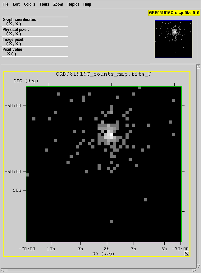
One readily observes that there are many pixels containing a few counts each near the burst location, and few pixels containing any counts away from the burst. It is also evident that the burst location is not centered in the counts map. This means the preliminary location sent out in the GCN was not quite the right location. This is not uncommon for automated transient localizations.
Using ds9 instead of fv allows us to find the location of the brightest pixel, and a better position for the burst.
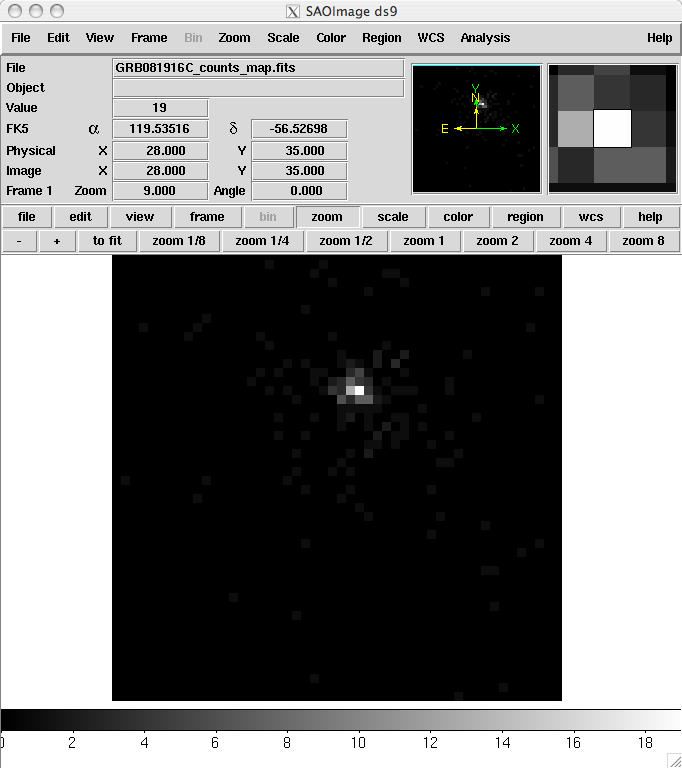
By simply mousing over that pixel, the RA and Dec of the likely burst location get displayed in the FK5 boxes (here, the new position is 119.5, -56.5). This is a quick method of localizing a burst, though not as accurate as fitting the data (described in the Likelihood Tutorial).
Note: To change the ds9 display for the mouseover from sexagesimal (the default) to degrees, go to the WCS menu and select "Degrees" in the bottom portion of the menu.
To look at the lightcurve:
- Open GRB081916C_light_curve.fits in fv.
The lightcurve is in the RATE extension. Choose 'All' to view the content of that extension. The extension has 4 columns: TIME, TIMEDEL, COUNTS and ERROR.
The time bins were created to have a width of 10 seconds, and therefore TIMEDEL is always 10.
- Now plot the COUNTS as a function of TIME. Select 'Plot' for the RATE extension. Click on 'Time' then on 'x'. Click on 'Counts' then on 'y'. Finally click on 'Plot'. The result is:
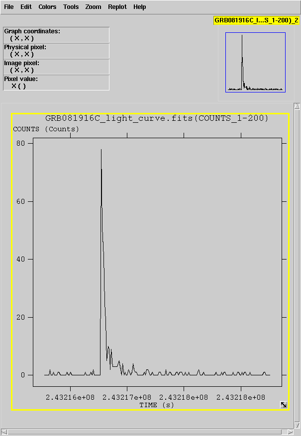
Note: Except for the period of the burst, almost all bins have 0-5 counts. This demonstrates that there is very little background for LAT observations of gamma-ray bursts.
Last updated: Nestor Mirabal 10/04/2018

- Curator: J.D. Myers
- NASA Official: Elizabeth Hays
- Fermi FAQ, Comments, Feedback
- › Privacy Policy and Important Notices
- › Accessibility
- › Contact NASA
- › Page Last Updated: Fri, Sep 05, 2025