GTBURST
This tutorial provides a step-by-step guide to using the gtburst GUI for GRB and solar flare analysis of GBM and LAT data. You can also watch a video tutorial
What it is used for?
- GBM data:
- download data from the GBM Trigger catalog, select data analysis interval, and interactively fit the background
- write out pha and rsp files for spectral analysis in either XSPEC or RMFIT
- LLE data:
- download data from the Fermi LAT Low-Energy Events Catalog, select data analysis interval, and interactively fit the background
- write out pha and rsp files for spectral analysis in either XSPEC or RMFIT
- LAT data:
- download photon events and spacecraft data from the LAT Data server
- produce navigation plots to allow user to select optimal time intervals and zenith cuts
- do photon selections based on energy, Region Of Interest (ROI), time, zenith, event class
- produce counts maps
- do likelihood analysis given a simple spectral model and background models
- localization using gtfindsrc or a TS map
- writes out pha and rsp files for spectral analysis in either XSPEC or RMFIT
Prerequisites
- Internet connection
- Recent version of gtburst
- latest installation of the Fermitools
Updating gtburst
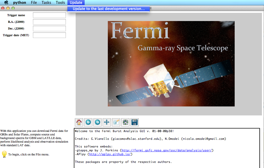
Before starting this analysis thread, make sure you have the latest version of gtburst. Gtburst adopts a "release early, release often" model, thus it is a good habit to check often for updates. Gtburst can be easily updated via the Update functionality. Menu: Update -> Update to the latest version.
This syncs with the github repository. You may need to sync twice initially to get to the latest version. After each update, you'll need to restart gtburst, which is automatically prompted.
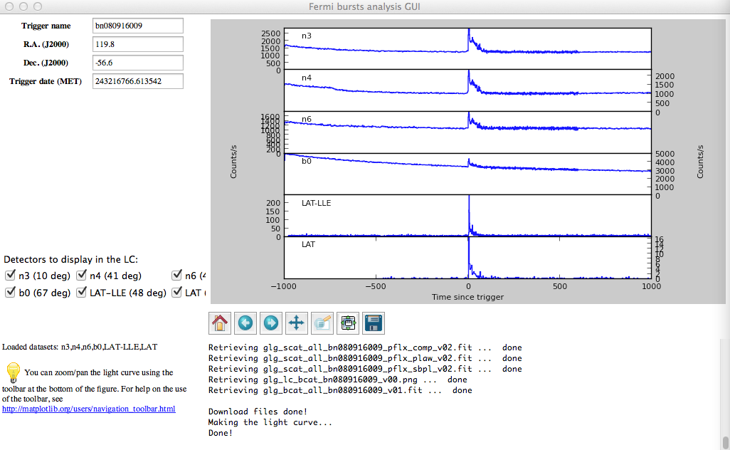
The interface and the log file
- A menu bar at the top.
- A parameter form on the upper left corner.
- A figure canvas on the upper right corner, which will contain graphical output from the various commands. You can always zoom and save the content of the figure canvas by using the toolbar at the bottom of it. You can find a description of the icons at: http://matplotlib.org/1.4.0/users/navigation_toolbar.html
- A help window on the lower left corner. You should always read what is contained here, since it gives you hints on what you are supposed to do at any step of the analysis.
- A console window which will contains the parameters of all commands run by the interface, as well as their outputs. Everything is contained here is also saved for your reference in the gtburst.log file in the directory where the program is running.
Immediate help from the interface
- At any step in any analysis task, you can read in the lower left corner a description on what you are supposed to do and some hints about things to keep in mind.
- If you don't remember what a given parameter in a command means, you can always click on the question mark "?" on the right of the parameter to get a short description of its meaning.
Analysis of a Gamma-Ray Burst
For this thread, we will analyze GRB080916C, one of the brightest LAT GRBs on record. All outputs from GUI window are in gtburst.log.
Start GTBurst
Open a terminal, and cd into a directory where you wish the gtburst output files to go. You may wish to make a sub directory specific to the object being analyzed to keep files organized (e.g. GRB080916C).
Type gtburst at command line.
Downloading data
Gtburst can download GBM, LLE, and LAT data from the FSSC, can be run on datasets previously downloaded, or can be loaded as a custom dataset.

Download datasets ...
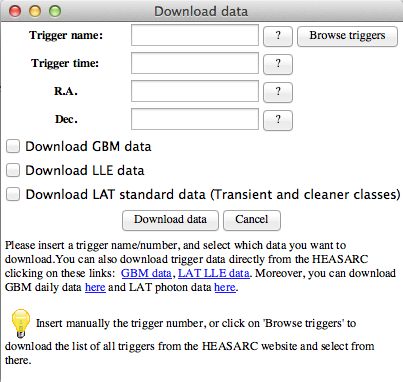
The trigger details can either be entered manually, or retrieved from the trigger catalog which includes both Swift-BAT and Fermi-GBM triggers.
Click "Browse triggers"
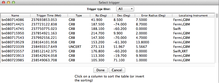
Triggers can be sorted by any of the columns by clicking on the header, or filtered by trigger type.
Note: GBM triggers may not appear immediately in this database, as they depend on the GBM team populating the table, which is done within 48 hours of the trigger.
Select the trigger and click Done (bn080916009 for GRB 080916C in this example).
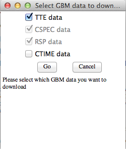
A box will pop up to confirm data selection. Time Tagged Events (TTE) versus binned CTIME data. TTE data files have finer time resolution and are therefore larger, and can be binned as needed.
GBM & LLE Data Analysis
A box will pop up to select the datasets for the following analysis. The number of degrees in parentheses is the angle from the individual detector boresight to the GRB. By default, the 3 or 4 smallest angle NaI's, the 1 smallest angle BGO, and LAT & LLE data will be selected. The backgrounds will be fit and spectral files created for only the selected detectors. The user may select additional detectors.
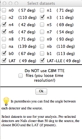
Light curves of the selected detectors with be created.
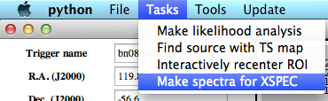
Make spectra for XSPEC
We will walk user through background and source selection, and output rsp & pha files.
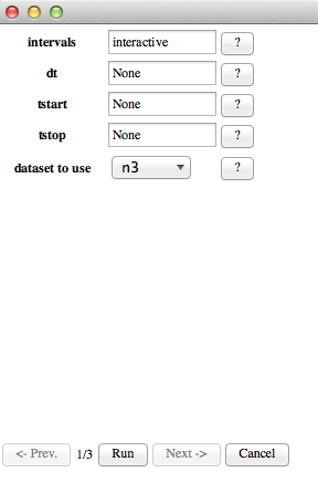
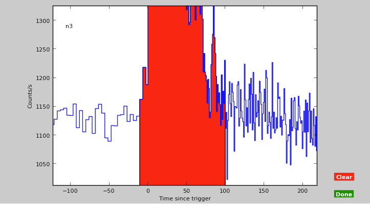
By default, the user will click to select the time intervals for source and background selection. The source interval will be chosen only once for the first detector used, which is the smallest angle NaI by default (n3 in this example).
Click Run to select interactively.
Zoom into the GRB emission using the ![]() button, and drawing a box around the GRB emission. Click the
button, and drawing a box around the GRB emission. Click the ![]() button again to exit the zoom feature. At any time, click
button again to exit the zoom feature. At any time, click ![]() to zoom back out. You can repeatedly refine the box smaller. Once zoom sufficiently, click once at the beginning of the interval, and again at the end. Once you are happy with the selection, click Done.
to zoom back out. You can repeatedly refine the box smaller. Once zoom sufficiently, click once at the beginning of the interval, and again at the end. Once you are happy with the selection, click Done.
Background fitting - click next, and then Run to interactively fit the background. Now zoom in to a region around the burst emission to fit the background. A few hundred seconds or so before and after the burst is usually sufficient. Select one interval prior to the burst (by clicking at the beginning and end) and another interval after the burst, where the background is approximately flat. Then click Done.
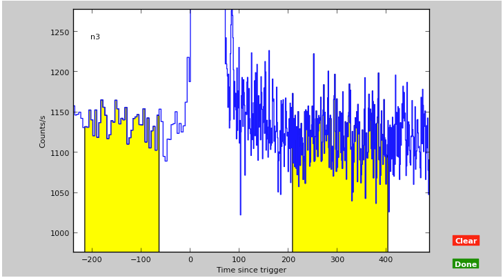
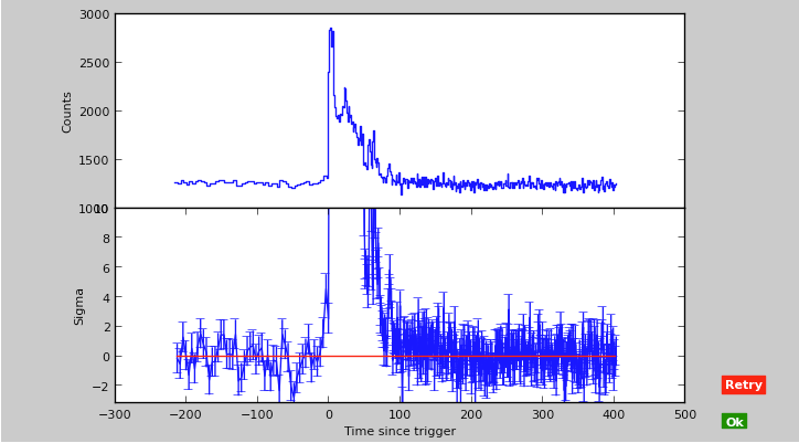
An automated fit to the background, which fits various polynomials is performed, to find the best fit. A plot showing the background-subtracted light curve is produced. If you are happy with the result, click OK, otherwise Retry to select new background intervals.
You will now need to produce a background fit for each subsequent detector. The same source interval is assumed. Redo e-f for each detector including BGO & LLE.
When all detectors are completed, click Next, and then Run to produce the output files, and Finish to go back to the starting menu. The directory where you're running gtburst should now contain the following files, which can be read into XSPEC to conduct a joint spectral fit as described in http://fermi.gsfc.nasa.gov/ssc/data/analysis/scitools/combined_LAT_GBM.html
bn080916009_n3_srcspectra.pha
bn080916009_n3_weightedrsp.rsp
bn080916009_n3_bkgspectra.bak
bn080916009_n4_srcspectra.pha
bn080916009_n4_weightedrsp.rsp
bn080916009_n4_bkgspectra.bak
bn080916009_n6_srcspectra.pha
bn080916009_n6_weightedrsp.rsp
bn080916009_n6_bkgspectra.bak
bn080916009_b0_srcspectra.pha
bn080916009_b0_weightedrsp.rsp
bn080916009_b0_bkgspectra.bak
bn080916009_LAT-LLE_srcspectra.pha
bn080916009_LAT-LLE_weightedrsp.rsp
bn080916009_LAT-LLE_bkgspectra.bak
LAT Data Analysis
After downloading a dataset or loading data from a directory, it's best to start with the navigation plot.
Click Tools->Make navigation plots
![]()
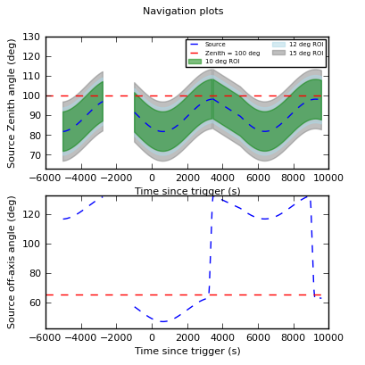
The navigation plots will pop up in a separate window. The upper plot is the angle between the GRB RA/Dec and the Fermi zenith angle. This indicates when the GRB is and is not occulted by the Earth. A zenith angle cut of 100 is fairly standard for a GRB, but can be adjusted slightly higher if the source is very bright at that time, or lower if the source is fainter and the user is concerned about Earth limb contamination.
The lower panel of the navigation plot is the angle between the GRB RA/Dec and the boresight of the LAT. This indicates when the source is within the LAT FoV. The size of the LAT FoV is dependent on energy and event class.
The navigation plots are in reference to the GRB localization in the GBM GRB catalog, which may be the best available GBM position (~few deg), an announced LAT position (~0.1-1 deg), or a much more accurate position from follow-up (~arcsec). The user can manually adjust the position in the GUI window at this time, or later based upon the counts map. If the user changes the R.A. and Dec. in the initial window, making the navigation plots again will update the plots using the new position.
Likelihood Analysis
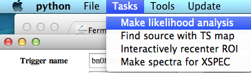
Click Tasks->Make likelihood analysis
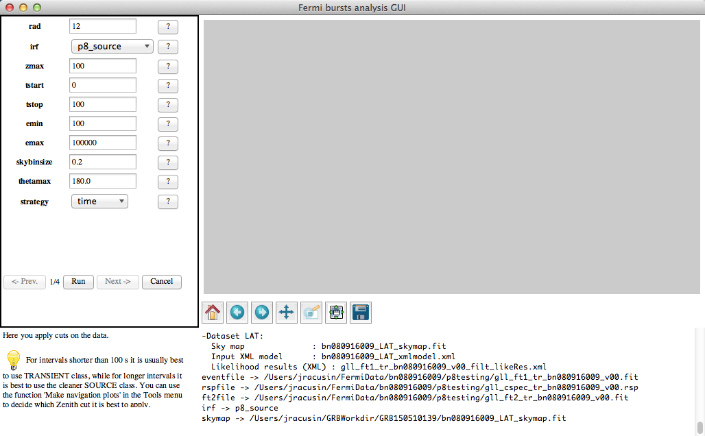
The first step is filtering for the counts map, which can be repeated and optimized. The parameters:
| Parameter | Description |
|---|---|
| rad | Radius of interest (degrees). Customary values correspond to the 95% containment of the PSF at the `Emin` energy. If you use `Emin=100 MeV`, `rad` should be 12 degrees for any Transient class and 10 degrees for Source or cleaner classes. |
| irf | The event class. In GRB analysis, the transient class is usually sufficient for short (< 100 seconds) timescales and spectral analysis, while source class is preferred for longer intervals and localizations. Event Class recommendations for different analyses are discussed at: LAT DP Documentation. |
| zmax | Zenith angle cut. If the parameter `strategy=time` (default), any time interval where any part of the ROI is at a Zenith angle larger than `zmax` is excluded. This is the normal choice for GRB and SF analysis. If `strategy=events`, all events with a Zenith angle larger than `zmax` will be excluded. Using `strategy=events` can introduce systematic uncertainties in the analysis, so caution is advised. |
| Tstart | Time to start analysis relative to GRB trigger. This can be specified either as a time from the trigger time or as a Mission Elapsed Time (MET). The system will automatically interpret MET values properly. |
| Tstop | Time to stop analysis relative to GRB trigger. This can be specified either as a time from the trigger time or as a Mission Elapsed Time (MET). The system will automatically interpret MET values properly. |
| Emin | Minimum energy for analysis in MeV. The standard value is `100 MeV`, as going below that requires special attention. |
| Emax | Maximum energy for analysis in MeV. |
| Skybinsize | Binning for map. |
| Thetamax | An additional cut that excludes time intervals in which the source position is more than `Thetamax` degrees from the center of the LAT field of view. Useful for bright bursts to reduce errors on localization but usually not necessary to adjust. |
| Strategy | Method of zenith angle cut. Using `strategy=time` (default) excludes all time intervals where any part of the ROI has Zenith angles larger than `zmax`. Avoid changing this value unless necessary. `strategy=events` excludes all events with Zenith angles larger than `zmax`, but can introduce subtle systematic errors. |
Using strategy=time (the standard value) will exclude from the analysis all time intervals in which any part of the ROI is at Zenith angles larger than the zmax value. Do not change this value unless you know what you are doing! Using strategy=events will exclude from the analysis all events with a Zenith angle larger than zmax, which can introduce subtle systematic errors in the analysis difficult to judge.
Click Run
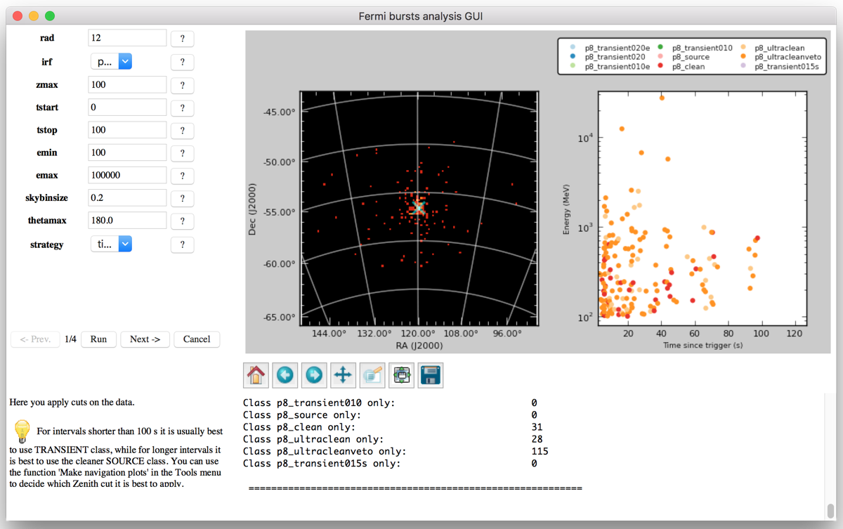
You will then see the resulting counts map and photon energy as a function of time. You can click on photons on the right plot, which will be highlighted on the left plot with a small white circle. This is helpful for determining if a particular high energy photon is clustered near others. A small text box will also appear with the ID of the run in which the event was detected, the event ID, the Zenith and the off-axis (theta) angle of that event. You can also zoom in the left plot, and only the photons within your zoomed area will remain in the right plot. This is useful for example to figure out which photons are close to the source position. Note that f you zoom in the right plot, the left plot will NOT change since this would require a new run of the command.
Click Next
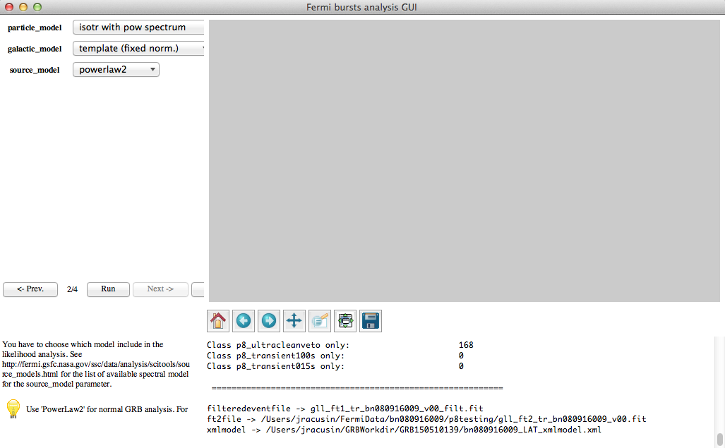
Next we choose the components of our likelihood model. This command will produce a XML file containing your likelihood model, as described here (add a link to the likelihood tutorial). For source class, a particle model of isotr template is appropriate. The other defaults are sufficient. Click Run, once that finishes, click next.
Gtburst will automatically add nearby bright catalog sources to your XML file. Once the dialog box finishes, click Run.
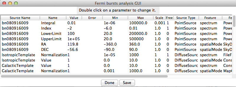
A window summarizing the fit parameters of the model will pop up. You can modify the parameters (e.g. fixing index to some value), or simply click Done to leave everything as it is. If you make changes, be sure to click save, and click Done when finished. Then, once the window with the list of parameters is closed, click Next.
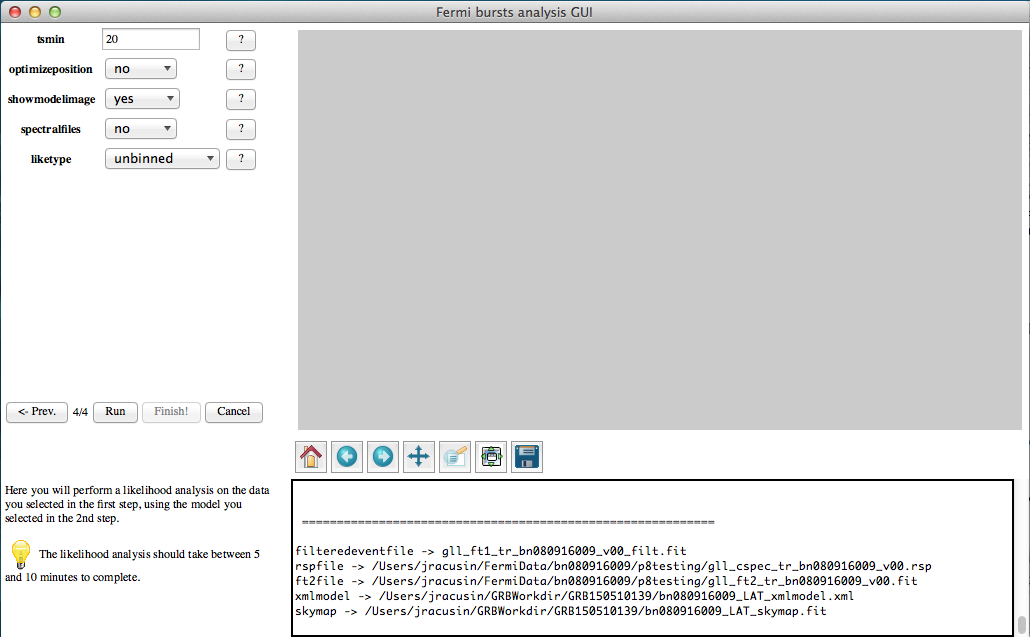
Now you will be given options on the outputs of the likelihood analysis. Optimizeposition=yes will call gtfindsrc at the end of the likelihood analysis and attempt to improve the GRB localization. Showmodelimage=yes will create a model map and display it. This does not have any impact on the actual analysis, but allow you to see a representation of your final model. Spectralfiles=yes will create the pha and rsp files necessary to do spectral analysis in XSPEC or rmfit. Each of these steps will make the analysis take longer. Click run.
Results
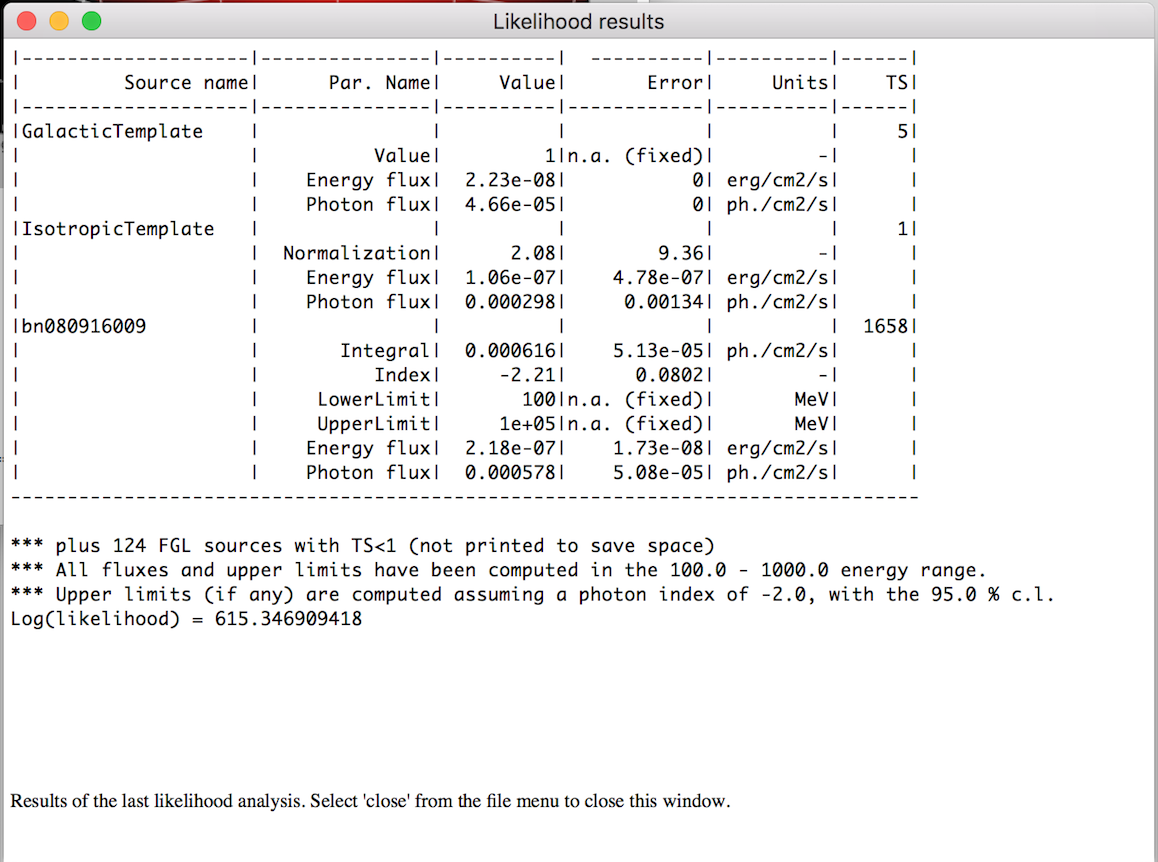
Likelihood fit result parameters of GRB, relevant nearby sources, and background models. You must close this window to proceed.
Resulting count map and likelihood model image. GRB 080916C is well detected!

If a substantially improve position is available, enter this position in the start window, which can be reached by clicking Finish, then repeat likelihood analysis from that position.
TS map
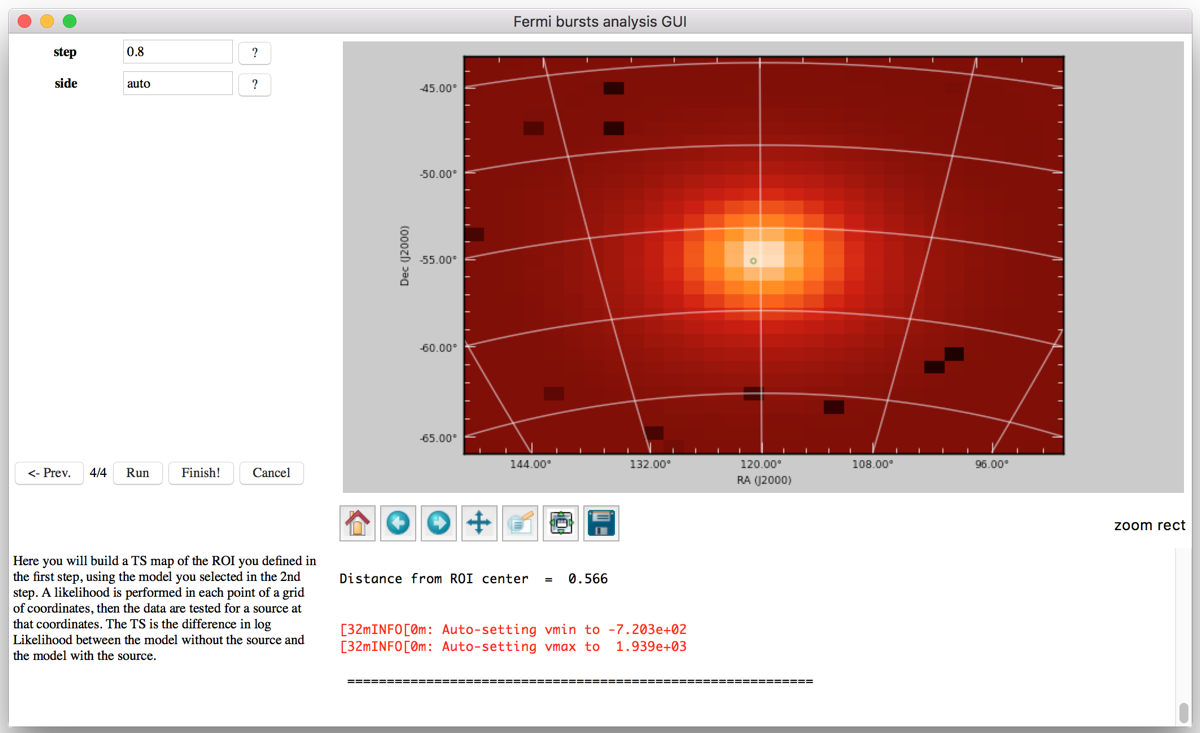
If photon clustering isn't entirely obvious or to potentially improve the localization further, one can create a TS map, which can take a while to run, especially on a long dataset. For very bright GRBs, note that the binning may be more of a limiting factor then the photon statistics on localization determination.
Tasks->Find source in TS Map
Follow similar steps as the likelihood analysis, ending up with a map and localization. For GRB 080916C, the localization is not improved by the TS map because the statistical error is smaller than the TS map binsize.
Choose new center for likelihood analysis, useful for localizing a GBM burst, based upon visual determination of the position of the cluster of photons in the counts map.
Tasks -> Interactively recenter ROI
Make photon selections, click Run. Once it finishes, click Next, and Run.
Click on a new center position on the left counts map. Click Run, and finish. Then repeat the likelihood analysis step at this new location.