
Please Note: An updated, and maintained, version of this content is available on Github as a Jupyter notebook.
Pulsar Gating Tutorial
You may be looking at a supernova remnant, or seeking new pulsar wind nebulae, and need to remove the accompanying pulsar. Or you could be looking at starburst galaxies at higher galactic latitudes, and a pesky millisecond pulsar keeps getting in your way.
Pulsar gating is the process of removing the flux of a bright pulsar from a region of interest, thus enabling the analysis of fainter sources in the region. You can accomplish this by assigning pulse phases to the pulsar by using a known ephemeris. You will also need to use the pulsar light curve to define an off-pulse interval in phase-space. Once the phases are assigned, you can use gtselect to filter out the unwanted phase periods, effectively removing the pulsar from the data completely.
You can download this tutorial as a Jupyter notebook and run it interactively. Please see the instructions for using the notebooks with the Fermitools.
Step 1: Extract your data
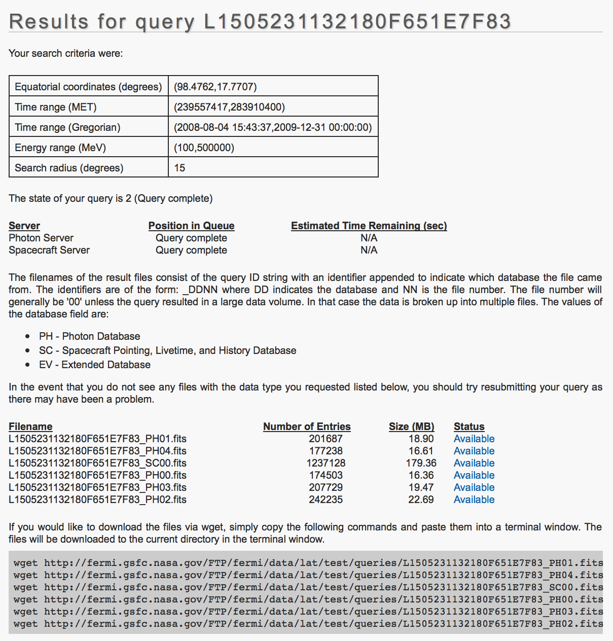
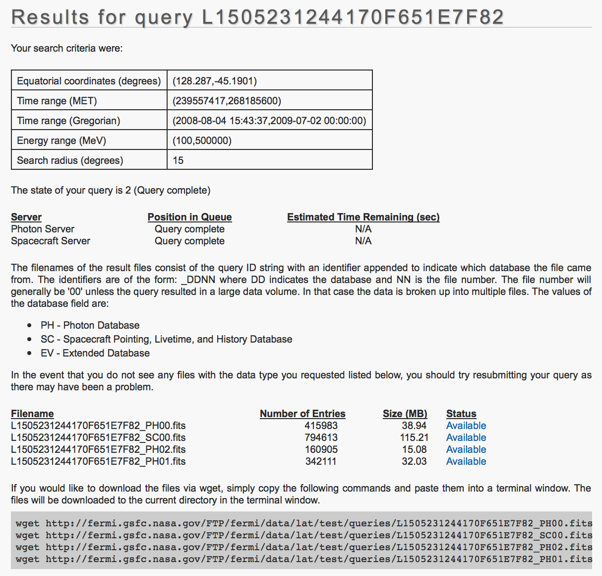
For this tutorial, we assume you know how to extract your data, prepare your data for analysis, and explore your data. First, lets take a look at a set of data that contains a bright pulsar. We'll use the pulsar Geminga (98.476204, 17.770661) with a 15° ROI, and the time range from the START of the mission to MJD 55196 (these position and time range are designed to match the data in the ephemeris file used in the next step). Geminga is very bright in the LAT, so you will get several event files to cover the full time span.
Below, we extract the Geminga data from the LAT Data Server.
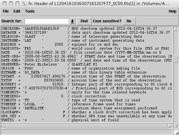
Next, we want to use gtselect to merge the event files and make the zenith cut. The data server already trims 30 seconds off each end of the LAT data to ensure that the spacecraft file will contain entries beyond both ends of the data, which is necessary for proper use of the pulsar tools. You can find the start and end times of the full dataset by looking at the TSTART and TSTOP keywords in the header of the spacecraft file.
Run gtselect. Here, Geminga.txt is a listing of all the event files to allow them to be merged. The spacecraft file (*SC*) has been renamed to spacecraft.fits for simplicity.
> gtselect evclass=128 evtype=3


Input FT1 file[] @Geminga.txt


Output FT1 file[] Geminga.fits


RA for new search center (degrees) (0:360) [] INDEF


Dec for new search center (degrees) (-90:90) [] INDEF


radius of new search region (degrees) (0:180) [] INDEF


start time (MET in s) (0:) [] INDEF


end time (MET in s) (0:) [] INDEF


lower energy limit (MeV) (0:) [] 100


upper energy limit (MeV) (0:) [] 500000


maximum zenith angle value (degrees) (0:180) [] 90


Done.
Then run gtmktime to update the GTIs, otherwise the exposure calculation will be off. While gtmktime can compensate for some exposure changes, it does not handle phase cuts. So you will need to scale any outputs from the analysis by hand. We'll talk about how to do that at the end of this tutorial.
> gtmktime


Spacecraft data file[] spacecraft.fits


Filter expression[] (DATA_QUAL>0)&&(LAT_CONFIG==1)


Apply ROI-based zenith angle cut[] no


Event data file[] Geminga.fits


Output event file name[] Geminga_gtis.fits
Next use gtbin followed by ds9 to take a look at the data:
> gtbin


Type of output file (CCUBE|CMAP|LC|PHA1|PHA2|HEALPIX) [] CMAP


Event data file name[] Geminga_gtis.fits


Output file name[] Geminga_cmap.fits


Spacecraft data file name[NONE] spacecraft.fits


Size of the X axis in pixels[] 300


Size of the Y axis in pixels[] 300


Image scale (in degrees/pixel)[] 0.1


Coordinate system (CEL - celestial, GAL -galactic) (CEL|GAL) [CEL]


First coordinate of image center in degrees (RA or galactic l)[] 98.4756


Second coordinate of image center in degrees (DEC or galactic b)[] 17.7703


Rotation angle of image axis, in degrees[0.]


Projection method e.g. AIT|ARC|CAR|GLS|MER|NCP|SIN|STG|TAN:[] CAR


> ds9 Geminga_cmap.fits &
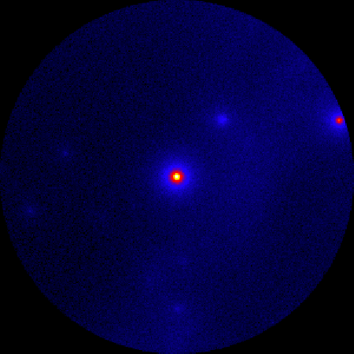
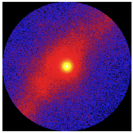
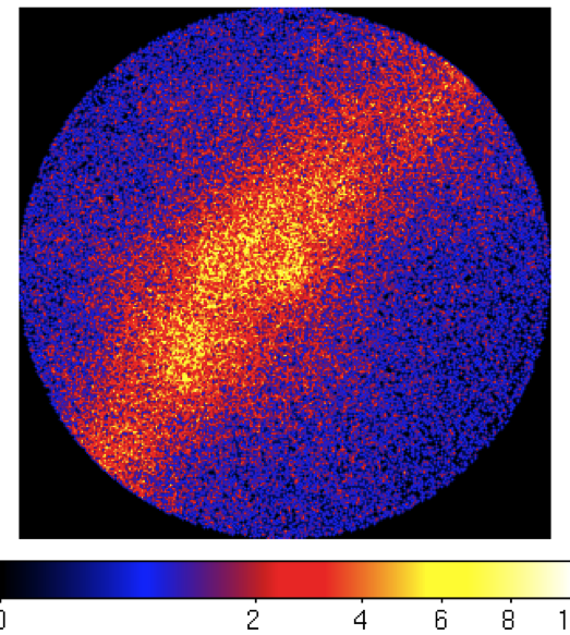
Here is the counts map showing a very bright Geminga centered in the ROI.
Step 2: Finding the pulsar ephemeris.
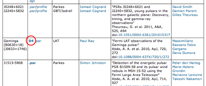
Now you have data with a very bright pulsar in it, and you need to remove this pulsar from your data. To do so, you have to find out a few things about that pulsar. This information can be found in the pulsar's ephemeris file and in any accompanying paper, both of which can be found at the LAT Data Access → LAT Pulsar Ephemeris page:
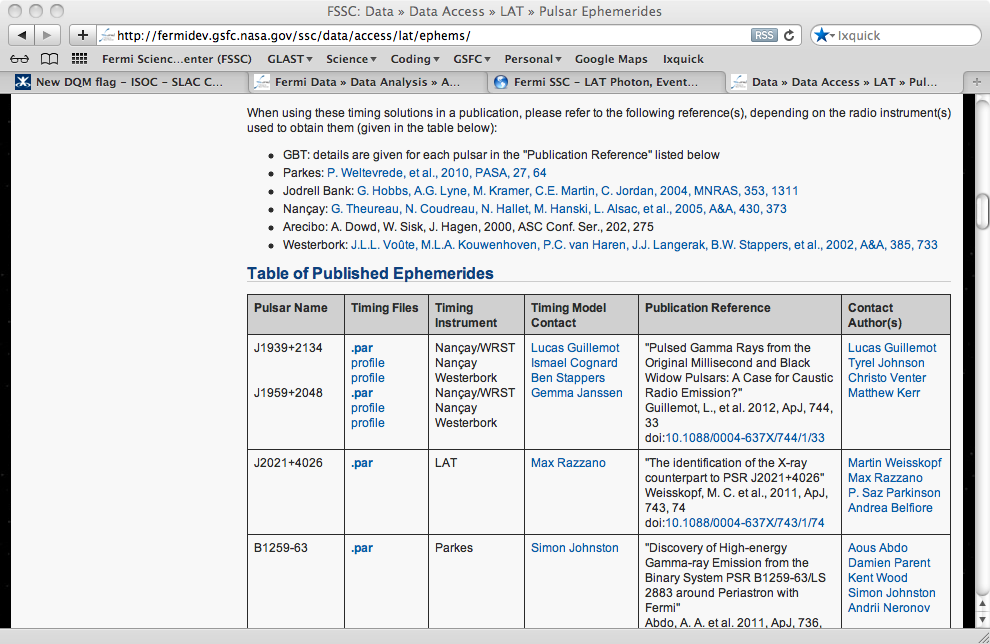
This page contains the ephemerides that have been used by the LAT team for their published papers to date. It provides several useful bits of information; the ephemeris file for each pulsar, the timing contact (i.e. the person who actually calculated the ephemeris), links to each paper (papers are likely to contain light curves for each pulsar), and finally the contact authors for each paper. If you have questions about the ephemeris itself, you should contact the timing contact. For question about light curves and interpretation of the pulsar data, contact the paper's contact authors. All email addresses use "at" for the @ symbol, and "dot" for the periods, just to keep email addresses less obvious on the open internet. You'll have to correct those before you send any emails.
The ephemeris files themselves are listed in the "Table of Published Ephemerides" under the "Timing Files" heading. There are two types of ephemeris files; .par files, which are used for the TEMPO2 tool, and D4 files which are used by the Fermitools. As a note, the TEMPO2 tool is not associated with the FSSC. However, members of the LAT instrument team have provided specialized files to allow LAT data to interface with that toolset.
Let's download an ephemeris file and see what it looks like. Scroll to the first row of the table that contains a D4 in the second column. This should be the pulsar Geminga, a bright gamma-ray pulsar that is radio quiet. If you open the .par file associated with Geminga using a text viewer, you will see some important information:
- Pulsar name and position — these positions are typically determined by the timing data, but sometimes come from X-ray or radio interferometric observations. For some pulsars there may be proper motion (PMRA, PMDEC) or parallax (PX) values as well.
- Spin information — this gives the primary spin frequency (F0), and one or more derivatives (note that the spin frequency is equal to F0 at PEPOCH). The first derivative (F1) is the rate at which the pulsar is slowing down and is dominated by the secular spindown of the pulsar. Any higher order derivatives are usually dominated by timing noise. If the pulsar you are looking at is in a binary, you will also see orbital parameters in this section. Some par files include "WAVE" terms, which are used to model timing noise using harmonically related sinusoids (Hobbs et al. 2004).
- START and FINISH — These provide information about the time period over which the ephemeris is good. Some pulsars (particularly millisecond pulsars) are very stable, and an ephemeris can be safely extrapolated for months beyond the FINISH time. However, many gamma-ray pulsars have significant timing noise or glitches, which make it very unsafe to extrapolate. If you see frequency derivatives of F2 or higher or WAVE parameters in the PAR file, DO NOT use it beyond its valid dates! If you cannot find an ephemeris that covers the time span you need, email the timing contact to find out if there is something more recent.
- The TZRMJD, TZRFRQ, and TZRSITE paramaters define phase 0.0 for the ephemeris. The fiducial point on the radio profile arrived at TZRSITE at frequency TZRFRQ at the moment TZRMJD. Often, but NOT always, the fiducial point on the radio profile is the peak, but you must always ask the person who made the ephemeris to be sure, because other conventions are used!
* WARNING: If your PAR file comes from Tempo2 (usually you can tell by "EPHVER 5" in the file), then the default time system is TCB, NOT TDB! Tempo2 only uses TDB if there is "UNITS TDB" in the par file. This is VERY important if you feed the values in the par file to a program that expects TDB, such as tempo1 or the D4 FITS files.
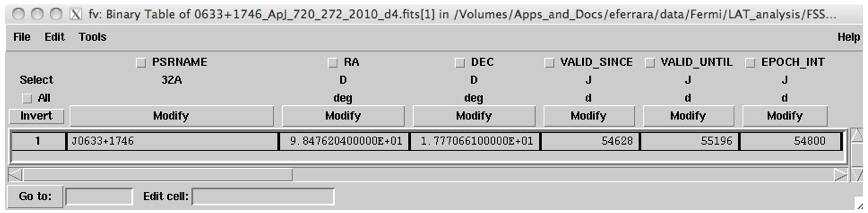
This same information is included in the D4 file, but in FITS format rather than text. Download the D4 ephemeris file for Geminga to your working directory.
Step 3: Assigning pulse phases
Now that you have the ephemeris, you need to use this information to assign pulse phases to the events in your data file.
Run gtpphase to add a column containing pulse phases to your events file. It may be advisable to save off a backup copy of your events file before running this tool, as it permanently modifies the input file.
> cp Geminga_gtis.fits Geminga_gtis.fits.backup


> gtpphase


Event data file name[] Geminga_gtis.fits


Spacecraft data file name[] spacecraft


Pulsar ephemerides database file name[] 0633+1746_ApJ_720_272_2010_D4.fits


Pulsar name[] J0633+1746


How will spin ephemeris be specified? (DB|FREQ|PER) [DB]
The pulsar name needs to match the value in first column of the D4 ephemeris file. Here, Geminga is actually called "J0633+1746" in the file.
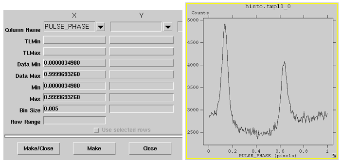
The file Geminga_gtis.fits will now have a new column, PULSE_PHASE, which you can use to filter your data. But it's always wise to check, so verify the data looks good by creating a quick folded light curve using the FV histogram function. Here I have used a bin size of 0.005 in phase space. You should see two strong peaks from the pulsar, with noise between the peaks. That noise is the data we're interested in. The peaks are the pulsed flux that we wish to remove, which we will discuss in the next step. If you don't see this pattern, you may have made a mistake in assigning phases.
If you want to assign pulsar phases with the Fermitools but don't have a D4 database file, you can use gtpphase and enter the timing parameters from the .par file by using the "FREQ" option.
> cp Geminga_gtis.fits.backup Geminga_gtis_par.fits


> gtpphase


Event data file name[] Geminga_gtis_par.fits


Spacecraft data file name[] spacecraft.fits


Pulsar ephemerides database file name[] none


Pulsar name[] J0633+1746


How will spin ephemeris be specified? (DB|FREQ|PER) [] FREQ


Epoch for the spin ephemeris[] 54800


Time format for spin ephemeris epoch (FILE|MJD|ISO|FERMI|GLAST) [] MJD


Time system for spin ephemeris epoch (FILE|TAI|TDB|TT|UTC) [] TDB


Right Ascension to be used for barycenter corrections (degrees)[] 98.476204


Declination to be used for barycenter corrections (degrees)[] 17.770661


Base value of phase at this epoch[0]


Pulse frequency at the epoch of the spin ephemeris (Hz) (0.:) [] 4.2175670649262114748


First time derivative of the pulse frequency at the epoch of the spin ephemeris (Hz/s)[] -1.9525033316064710553e-13


Second time derivative of the pulse frequency at the epoch of the spin ephemeris (Hz/s/s)[] 0
However, the Fermitools do not support phase assignment for pulsars with more than one WAVE term. So if your .par file has timing parameters at higher orders than F2, you will need to use TEMPO2 to assign pulse phases. A discussion of TEMPO2 phase assignment is available in the second section of this tutorial.
Step 4: Remove events from the pulsar
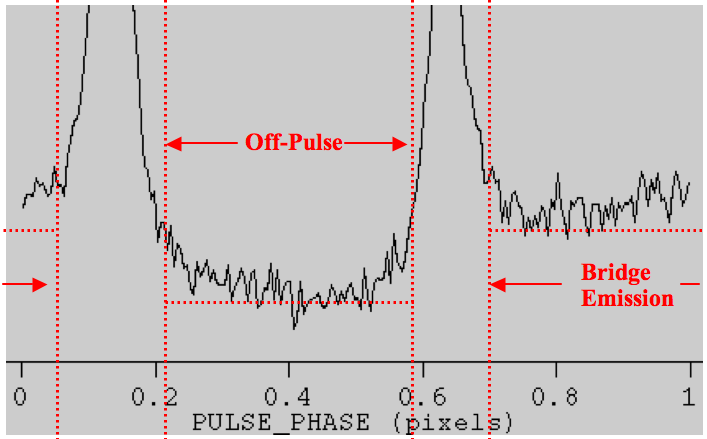
If you look closely at the light curve, you will see that during the period when the pulsar is not pulsing, there are still events coming in. These "off-pulse" events are the data you care about, so we want to filter out the pulsar "on-pulse" events. To do this, you define an "off-pulse" interval. The off-pulse could be both phase intervals between the pulses (in this case, .22-.58 and .72-.05). But some pulsars never turn off completely between the pulses. In fact, for Geminga you'll notice the background level after the second pulse is quite a bit higher than between the pulses. This higher level is called "bridge emission" and must also be removed in order to completely remove the pulsar. For pulsars with an interpulse, you will probably only be able to define a single off-pulse interval.
You might want to look at the LAT team paper at this point. For many of the sources, the people who did the pulsar analysis also defined on off-pulse period for the pulsar. In either case, pick what you think is the best off-pulse interval and move on to the next step. For this analysis we will use phases .22-.58 for our off-pulse period.
Once you have defined your off-pulse interval, use gtselect to filter out the unwanted events when the pulsar is ON.
> gtselect evclass=128 evtype=3 phasemin=.22 phasemax=.58


Input FT1 file[@Geminga.txt] Geminga_gtis.fits


Output FT1 file[Geminga.fits] Geminga_22_58_phasecut.fits


RA for new search center (degrees) (0:360) [] INDEF


Dec for new search center (degrees) (-90:90) [] INDEF


radius of new search region (degrees) (0:180) [] INDEF


start time (MET in s) (0:) [] INDEF


end time (MET in s) (0:) [] INDEF


lower energy limit (MeV) (0:) [] 100


upper energy limit (MeV) (0:) [] 500000


maximum zenith angle value (degrees) (0:180) [] 90


Done.
Note that phasemin and phasemax are not prompted parameters, so you will need to define them on the command line. If your off-pulse interval spans the ends of the phase assignment (as would be the case here if we used the interpulse region) you will need to extract two events segments corresponding to phases 0 to .05, and phases .72 to 1. gtselect does not handle multiple phase cuts, so you should consider using the FTOOL ftselect instead.
Step 5: Verify the pulsar is missing
Now you should bin your data again and check to see if the contribution from the pulsar is really gone. Use gtbin to bin the remaining data, and view it in ds9.
> gtbin


Type of output file (CCUBE|CMAP|LC|PHA1|PHA2) [CMAP]


Event data file name[Geminga.fits] Geminga_22_58_phasecut.fits


Output file name[Geminga_cmap.fits] Geminga_22_58_phasecut_cmap.fits


Spacecraft data file name[spacecraft.fits]


Size of the X axis in pixels[300]


Size of the Y axis in pixels[300]


Image scale (in degrees/pixel)[0.1]


Coordinate system (CEL - celestial, GAL -galactic) (CEL|GAL) [CEL]


First coordinate of image center in degrees (RA or galactic l)[98.476204]


Second coordinate of image center in degrees (DEC or galactic b)[17.770661]


Rotation angle of image axis, in degrees[0]


Projection method e.g. AIT|ARC|CAR|GLS|MER|NCP|SIN|STG|TAN:[CAR]


> ds9 Geminga_22_58_phasecut_cmap.fits &
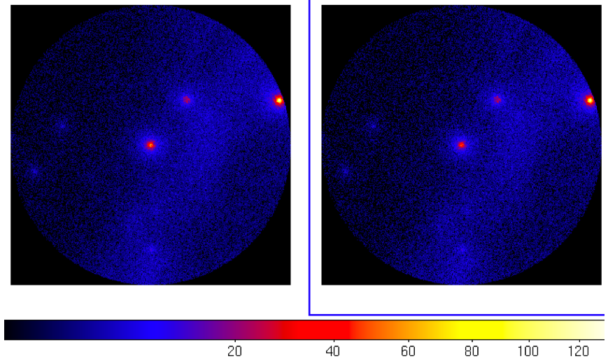
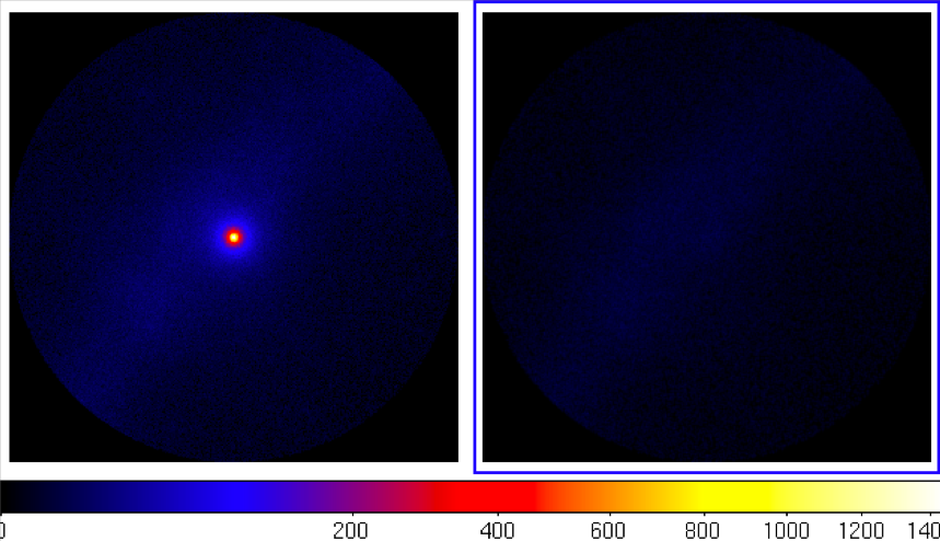
As you can see, the contribution from Geminga in the new map (left) is mostly gone. The fainter source near the edge of the ROI is now the strongest source in the field. What you will also notice is that you now have many fewer events. That's because the contributions from the other sources has been scaled down by the fraction of data you have removed; in this case the remaining data is 36% (58-22) of the original. This is, in effect, a cut in livetime on these sources.
You can adjust the cuts on phase to try to remove more and more of the pulsar, but this significantly affects the livetime of your other sources, so you should use these cuts with care. Here is a comparison between the previous phase interval of .22-.58 (left) and a tighter cut of .25-.55 (right). As you can see, the pulsar contribution is diminished, but not completely gone.
This data can now be used with a source model in a normal binned or unbinned likelihood analysis to find the flux of the fainter sources (you should still leave a source at the position of Geminga to absorb the residual flux since this pulsar never turns off completely). Once you have fitted your data, multiply the resulting fluxes by 2.778 (or 1/.36) to get the proper flux values for the sources.
While Geminga is not really close to other bright gamma-ray sources, regions like Cygnus or Carina contain multiple bright sources that lie very close together. Such regions may benefit significantly from the use of pulsar gating to remove pulsar contributions. However, be aware, every pulsar you remove costs a significant fraction of livetime. So use this technique sparingly.
Using TEMPO2 for phase gating
Since many young gamma-ray pulsars (like Vela) are very noisy, you may need to use TEMPO2, a pulsar analysis package developed by radio astronomers, to assign phases for more complex ephemerides. You can get all the information and download the TEMPO2 software at http://www.atnf.csiro.au/research/pulsar/tempo2/index.php?n=Main.HomePage.
A plugin designed to ingest LAT event data and export phase assignments is already included in the TEMPO2 package, so the software should be compatible with your LAT data file. Instructions on how to install and run the TEMPO2 package with the LAT plugin have been provided by the developer.
For TEMPO2 to run, the TEMPO2 environment variable must be set to the full path to the T2runtime directory. During installation you should specify that the plugins should be installed in this same directory. Otherwise, you will need to copy the plugins directory into this folder.
Here we use a recent Vela parameter file from the LAT Pulsar Ephemeris page. Checking the content of the .par file, we see the ephemeris is valid from MJD 54647.403 to MJD 55014.192. We download data from the LAT Data server corresponding to the pulsar position and covering most of that time range:
Like Geminga, Vela is very bright so we get several photon files that we need to combine, trim, and apply the zenith cut using gtselect. This step is always followed immediately by gtmktime:
> gtselect evclass=128 evtype=3


Input FT1 file[] @Vela.list


Output FT1 file[] Vela_events.fits


RA for new search center (degrees) (0:360) [] INDEF


Dec for new search center (degrees) (-90:90) [] INDEF


radius of new search region (degrees) (0:180) [] INDEF


start time (MET in s) (0:) [] INDEF


end time (MET in s) (0:) [] INDEF


lower energy limit (MeV) (0:) [] 100


upper energy limit (MeV) (0:) [] 500000


maximum zenith angle value (degrees) (0:180) [] 90


Done.


> gtmktime


Spacecraft data file[] spacecraft.fits


Filter expression[] (DATA_QUAL>0)&&(LAT_CONFIG==1)


Apply ROI-based zenith angle cut[] no


Event data file[] Vela_events.fits


Output event file name[] Vela_gtis.fits
Looking at the data, we see the very bright pulsar in the center of the field
> gtbin


Type of output file (CCUBE|CMAP|LC|PHA1|PHA2) [] CMAP


Event data file name[] Vela_gtis.fits


Output file name[] Vela_cmap.fits


Spacecraft data file name[] spacecraft.fits


Size of the X axis in pixels[] 300


Size of the Y axis in pixels[] 300


Image scale (in degrees/pixel)[] 0.1


Coordinate system (CEL - celestial, GAL -galactic) (CEL|GAL) [CEL]


First coordinate of image center in degrees (RA or galactic l)[] 128.836


Second coordinate of image center in degrees (DEC or galactic b)[] -45.1763


Rotation angle of image axis, in degrees[0]


Projection method e.g. AIT|ARC|CAR|GLS|MER|NCP|SIN|STG|TAN:[CAR]


> ds9 Vela_cmap.fits &
Assigning pulse phases
To assign pulse phases, first run TEMPO2 and check if the plugins are detected by:
> tempo2 -h
You should see "Fermi" included in the list of plugins at the end of the help file. To see what options are available with the Fermi plugin, type:
> tempo2 -gr fermi -h
To assign pulse phases to your FITS file, specify the Fermi plugin, the events (ft1) file, the spacecraft (ft2) file, and the ephemeris (-f). To add a column to the FITS file with the pulse phase, use the -phase flag. The -graph 0 flag suppresses the graphical output from the tool. The Fermi plugin for TEMPO2 was written by Lucas Guillamot, and a user's guide is available at the FSSC.
> tempo2 -gr fermi -ft1 Vela_gtis.fits -ft2 spacecraft.fits -f 0835-4510_ApJ_713_154_2010.par.txt -phase -graph 0


This program comes with ABSOLUTELY NO WARRANTY.


This is free software, and you are welcome to redistribute it


under conditions of GPL license.


Looking for /Volumes/Apps_and_Docs/eferrara/data/Fermi/LAT_analysis/tempo2/T2runtime/plugins/fermi_darwin_plug.t2


------------------------------------------


Output interface:    fermi


Author:              Lucas Guillemot


Updated:             16 November 2010


Version:             5.3


------------------------------------------


First photon date in FT1: 239562873.481502 MET (s)


 Last photon date in FT1: 268182488.766691 MET (s)


First START date in FT2:  239557417.494176 MET (s)


 Last START date in FT2:  268185623.600000 MET (s)


Setting waveepoch to 54800


Treating events # 1 to 5000...


Treating events # 5001 to 10000...


.


<output suppressed>


.


Treating events # 440001 to 445000...


Treating events # 445001 to 447975...


Done with J0835-4510
After viewing the lightcurve in fv, the off-pulse for Vela seems to be .68-.03. This will require two phase cuts (0-.03 and .68-1). Remember, gtselect does not handle multiple phase cuts, so we will use ftselect.
> ftselect ' Vela_gtis.fits[events]' Vela_phasecut.fits '(PULSE_PHASE > 0 && PULSE_PHASE < 0.03) || (PULSE_PHASE > 0.68 && PULSE_PHASE < 1)'
If you compare the number of events in the pre- and post-filter files, you should find the number of events remaining is about one quarter the original number. Since Vela is the brightest gamma-ray source in the sky, this is to be expected.
Now let's see what remains of Vela in our dataset:
> gtbin


Type of output file (CCUBE|CMAP|LC|PHA1|PHA2) [] CMAP


Event data file name[] Vela_phasecut.fits


Output file name[] Vela_phasecut_cmap.fits


Spacecraft data file name[] spacecraft.fits


Size of the X axis in pixels[] 300


Size of the Y axis in pixels[] 300


Image scale (in degrees/pixel)[] 0.1


Coordinate system (CEL - celestial, GAL -galactic) (CEL|GAL) [] CEL


First coordinate of image center in degrees (RA or galactic l)[] 128.836


Second coordinate of image center in degrees (DEC or galactic b)[] -45.1763


Rotation angle of image axis, in degrees[] 0


Projection method e.g. AIT|ARC|CAR|GLS|MER|NCP|SIN|STG|TAN:[] CAR


> ds9 Vela_phasecut_cmap.fits &
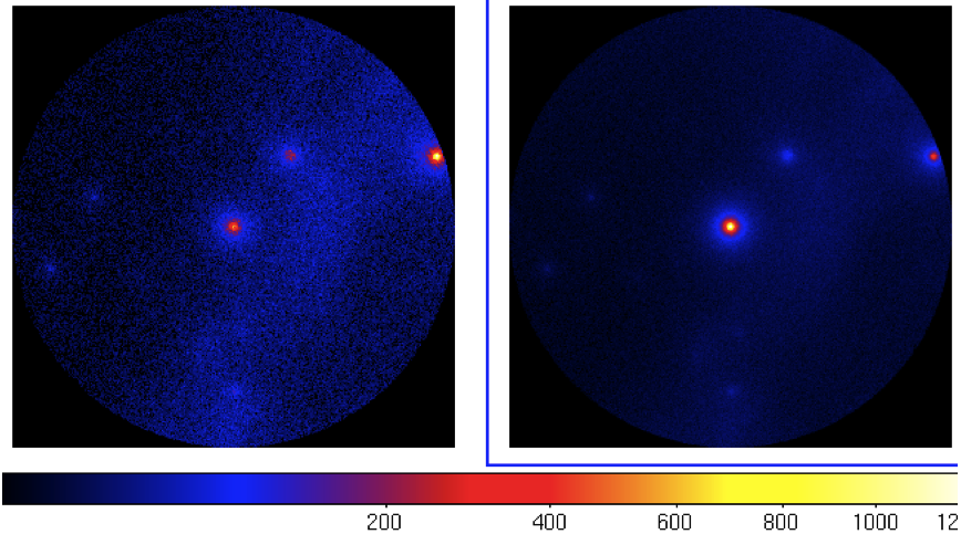
By adding another frame and scaling to have the same maximum value, we can compare what the region looks like with and without Vela.
This region contains several high-energy galactic sources that are difficult to detect under the strong galactic diffuse emission that is present. You can solve this by cutting out the low-energy events by using gtselect and changing the minimum energy to something higher, like 1 GeV.
> gtselect


Input FT1 file[] Vela_phasecut.fits


Output FT1 file[] Vela_phasecut_gt1gev.fits


RA for new search center (degrees) (0:360) [] INDEF


Dec for new search center (degrees) (-90:90) [] INDEF


radius of new search region (degrees) (0:180) [] INDEF


start time (MET in s) (0:) [] INDEF


end time (MET in s) (0:) [] INDEF


lower energy limit (MeV) (0:) [] 1000


upper energy limit (MeV) (0:) [] 500000


maximum zenith angle value (degrees) (0:180) [] 90


Done.


> gtbin


Type of output file (CCUBE|CMAP|LC|PHA1|PHA2) [] CMAP


Event data file name[] Vela_phasecut_gt1gev.fits


Output file name[] Vela_phasecut_gt1gev_cmap.fits


Spacecraft data file name[] spacecraft.fits


Size of the X axis in pixels[] 300


Size of the Y axis in pixels[] 300


Image scale (in degrees/pixel)[] 0.1


First coordinate of image center in degrees (RA or galactic l)[] 128.836


Second coordinate of image center in degrees (DEC or galactic b)[] -45.1763


Rotation angle of image axis, in degrees[] 0


Coordinate system (CEL - celestial, GAL -galactic) (CEL|GAL) [] CEL


> ds9 Vela_phasecut_gt1gev_cmap.fits &
If you smooth the image, you will see that the majority of the galactic diffuse emission has been removed. Now two circular features emerge; VelaX, the pulsar wind nebula powered by the gated pulsar, and Vela Junior, a supernova remnant in the lower left quadrant of the image.
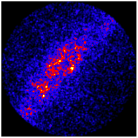
Both these sources lie along the galactic plane, and are completely invisible without using gating to remove the strong signal from the pulsar. To measure the significance of these two sources, you will need to perform an extended source analysis to fit the data to a template for each source. Don't forget that you have reduced the content of the data by a significant fraction. The remaining data is only 35% (100-68+3) of the original dataset. You will need to scale the flux results of any likelihood analysis by 100/35=2.857 to recover the flux of the sources from the original dataset.
Proper attribution
One final note: The collection and analysis of radio and LAT data that goes into generating each ephemeris is a significant time investment. Please be sure to acknowledge the source of the ephemeris and any appropriate references should you use any of these ephemerides for a publication. Please review the LAT Pulsar Ephemerides page for requested acknowledgements, email the timing contact for the pulsar ephemeris you have used, or contact the Fermi helpdesk if you have any questions regarding this policy.
Last updated by: Josefa Becerra - 06/07/2015

- Curator: J.D. Myers
- NASA Official: Elizabeth Hays
- Fermi FAQ, Comments, Feedback
- › Privacy Policy and Important Notices
- › Accessibility
- › Contact NASA
- › Page Last Updated: Mon, Sep 08, 2025