GBM Data Extraction and Gamma-Ray Burst Analysis
This section provides the information needed to obtain the GBM data as well as a step-by-step example of extracting and modeling a GBM Gamma-Ray Burst observation and fitting the data using the Gamma-Ray Spectral Fitting Package (RMFIT).
Prerequisites
- RMFIT, used as a spectral analysis tool starting in Step 2 of this procedure. (See Installing the GBM rmfit Tool.)
Assumptions
It is assumed that:
- You are in your work directory.
Note: For the purposes of this thread, the relevant burst properties are:
- T0 = 00:12:45.614 UT, 16 September 2008, corresponding to 243216766.614 seconds (MET)
- Trigger # 243216766
- RA = 121.8 degrees (= 08h 07m 12s)
- Dec = -61.3 degrees (= -61d 18m 00s)
- You have extracted the files used in this tutorial; these files can be found here. Alternatively, you could download the GBM data for 080916C as explained below.
- For analyzing GBM data, an alternative to RMFIT is XSPEC (see Xanadu Data Analysis for X-Ray Astronomy). The standard XSPEC analysis approach assumes that the background is approximately constant through the burst prompt emission and/or is negligible when compared to the burst emission. That is, this approximation is a valid in particular for bright and/or short bursts. RMFIT incorporates an interactive time-domain background fitting capability, and in comparison with XSPEC can thus produce significantly different results.
Steps:
- Retrieve the GBM data.
- Creating and viewing lightcurves.
- Background Selection and fitting.
- Source Selection.
- Spectral Analysis.
1. Retrieve the GBM data
The GBM consists of 12 NaI detectors (8 keV to ~900 keV) and 2 BGO detectors (200 keV to ~40 MeV). Each detector views a different portion of the sky so that, for a particular burst, there will be varying amounts of signal in the different detectors. The data can be obtained from the HEASARC BROWSE GBM Burst Catalog (the column explanation can be retrieved at the help file page). There are multiple ways of easily locating a particular burst based solely on its name; e.g., for GRB080916C, we can:
- search for "bn080916*" as the trigger name. The wildcard character * is needed as the GBM naming convention includes the fraction of day as well as the date; in this case, GRB080916C corresponds to bn080916009.
- search for "GRB080916*" as the name. We want GRB080916009 for the purposes of this tutorial.
- search for "2008-09-16" as any of the times.
After obtaining the search results, click on "D" next to the burst in question (GRB080916009) for the data products. The Quicklook Plot is a set of light curves for all 12 NaI detectors.
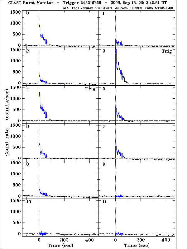
The GBM burst data include files for all detectors, whether or not they were oriented to accumulate many counts from a burst. As a rule of thumb, we want to use the 2 or 3 NaI detectors with the brightest signals (the NaI detectors that triggered should have accumulated the most burst counts, although if FERMI slews to point towards a long burst, other detectors will record significant burst flux). More detectors can be used, but for the most part, they will not increase the significance of the fits.
For this burst, we will choose NaI0 (which triggered), NaI3, and NaI4. Because we have chosen detectors between 0 and 5, we also select BGO0. If we had chosen NaI detectors 6-11, we would use BGO1. If both low- and high-numbered NaI are being used, then select both BGO detectors. More specific lightcurves can be found in the quicklook products directory.
In the page where the above set of light curves is located, you can select the "GBM Trigger Products (current)" directory to retrieve the full data for the all the detectors. They are sometimes updated to newer versions, indicated by the v0# numbers at the end of the file name (the version numbers are unimportant, and do not need to be consistent across the different files). The files for the NaI and BGO detectors are labelled differently: The corresponding files for the NaI detectors have n# (n0 to n9, na, or nb, with the last two corresponding to detectors #10 and #11) while for the BGO detectors BGO have b0 or b1. The naming convention for the GBM files can be found in the GBM Data Products page and in the Cicerone (See Data - GBM Data Products).
Instead of checking the above set of light curves, another way to select the triggered detector is from the burst data files. For example, look for the 'DET_MASK' keyword in the primary header of the file that begins "glg_trigdat" (use the FTOOLS fkeyprint to display the content of the keyword). This keyword provides a string that indicates which detectors triggered: the label "1" or "0" denotes if the NaI detector were triggered or not. Therefore, the string '000110000000' for 080916C means that NaI detectors 3 and 4 only were actually triggered.
For GRB080916C, the relevant files for the NaI detectors are:
- glg_cspec_n#_bn080916009_v0#.pha: The CSPEC spectral file (PHA2) for the GRB, binned into 1.024s time bins and 128 energy channels.
- glg_tte_n#_bn080916009_v0#.fit: The TTE (time-tagged event) data file for individual photons, binned into 128 energy channels.
- glg_cspec_n#_bn080916009_v0#.rsp: The instrument response file for each detector. These are used for both CSPEC and TTE data.
TTE files only cover ~300 s of data around the trigger time, and take longer to process. CSPEC files cover a longer time interval, and are good for longer events where the TTE files might not be sufficient for background fitting. The GBM team will update files as better data products become available. For example, response files may be updated as better burst positions become available (e.g., because Swift or the IPN provide a more accurate position that the GBM position).
In this tutorial, we will be analyzing the TTE data for NaI0. We will need the .fit file and the .rsp file.
2. Creating and viewing lightcurves
The TTE file contains information for each individual photon. We use RMFIT to view lightcurves:
prompt> rmfit

(Click on the IDL Virtual Machine dialog that comes up)


           				RMFIT 4.4.2

           A Lightcurve and Spectral Analysis Tool


           			Robert S. Mallozzi

           			Robert D. Preece

           			Michael S. Briggs

           			Adam M. Goldstein


           UNIVERSITY OF ALABAMA in HUNTSVILLE


           Copyright (C) 2000 Robert S. Mallozzi

           Portions (C) 2011 Robert D. Preece

           Includes portions of IDL Astronomy Users

           Library http://idlastro.gsfc.nasa.gov

           This program is free software; you can

           redistribute it and/or modify it under the

           terms of the GNU General Public License as

           published by the Free Software Foundation.
When RMFIT starts up, a box will appear that allows you to select FITS files in the directory specified by the current path. This directory may be one used in a previous RMFIT session, which is saved after exiting, so you may need to navigate to your working directory to select your data file. The main menu initially will contain the file filter *.fits (or your saved filter, usually *.lu) in the 'Select File(s) for Reading' box. If you enter the default filter, or enter another, a box will appear enabling you to choose any files matching the filter in the current directory.
Select data file glg_tte_n0_bn080916009_v0x.fit. Interacting with PHA data is done with the display window for the loaded file. Each loaded file typically has its own display window, with the file's name in the title. The first time a PHA data file has ever been opened in RMFIT, no lookup data exists and no selections have been made:
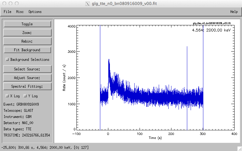
We suggest first examining the Spectral Display of counts per energy channel, which may be seen by typing 's', 't' or selecting the 'Toggle' button, if it is not visible. To select a portion of the energy range for fitting, type 'i' or choose the button "Select Source:/Source Interactive". Select the first bin in the range by positioning the cursor over a bin in the plot and clicking mouse button. Select the last bin in the same way. Numbers in the lower left-hand corner of the plot track the position of the cursor, which can be used if a particular value is to be selected. For the example GBM NaI FITS file, select approximately 8 to 900 keV, to avoid energy bins with electronic cut-off or overflow effects. Once the selection has been made (requires two clicks of the mouse), exit selection mode by moving the cursor to the left of the leftmost plot axis and clicking there (the numbers in the lower left hand corner should be replaced by the word 'EXIT').
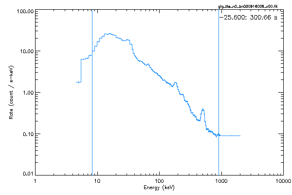
The bottom edge of the display should now read:
-25.920: 300.66 s, 8.201: 905.53 keV, [4: 124]
If you make a mistake, just make the selection again.
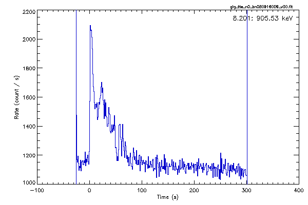
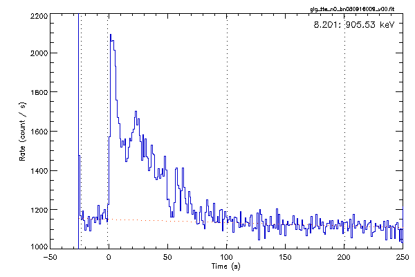
Toggle back to the lightcurve history display ('h', 't' or by selecting the 'Toggle' button). The displayed lightcurve is now integrated over the restricted range of the energy selection that was just made.
For GBM TTE data, the default time binning is 64 ms, which is somewhat noisy. Use the Rebin:->Temporal Resolution menu on the left hand side of the display to bring up the 'Rebin' dialog box. A good value to use for the next few steps is 1.024 s (the number entered here can have any value for TTE data; heed the warning for sub ms rebinning!). After entering this value and selecting 'OK', the rebinned lightcurve should appear.
In the same manner as the energy range was selected, we can select the region of interest where the burst flux is above background. To guide the eye for this selection, we suggest selecting and fitting the background model first.
3. Background Selection and fitting
The next task is to select a background model, using 'Fit Background'. Selection of the background is done in the same manner as the selection of energy bins, marking regions of interest with two mouse clicks. It is best to find regions both before and after the times containing the source counts. For the example file, we need at least two regions: roughly 20 s before the burst (at t = 0 s) and 100 s or so after. Try selecting both the regions -20 - -3 and +100 - +200 and then 'EXIT' to the left of the plot. RMFIT will request the order of the background model polynomial; choose 1. In the resulting chi-square plot, one can see that the scatter of the background fitting residuals is centered around the reduced chi-square value of 1. Dismiss the plot to accept the fit. Background fitting is an art form; for tips on how to select good background intervals and models, please see both the 'Tutorial' Help menu item (on the main RMFIT dialog) as well as the 'Background Fitting' Help menu item on each data display window.
4. Source Selection
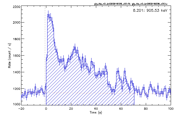
In order to select data for spectral fitting, we may first need to zoom in on the time history to see the details of the source counts. Type 'x' or select 'Zoom:/X Zoom' and then refine the plot by clicking on alternate sides of the source counts until the time region -20 - +100 s is displayed; 'EXIT' as usual. Follow the same 'Select Source:/Source Interactive' (or type 'i') routine as with the Spectral display, this time selecting the bright interval from +0 to +70 s. The selection is marked with cross hatching. The History display shows the rates for the selected energy range, '8.201: 905.53 keV' and the time range of the source intervals is indicated by the label, '0.0: 70.656 s'. (You may have to select the menu item 'Misc'->'Show Current Selections' first.) The dotted line at the bottom of the Burst History plot indicates the background model.
Toggling back to the spectral display for a moment, you can see both the background model and the selected source counts plotted together as histograms. One very good way of evaluating the background model is to look to see that there are no bins with large scatter in the background model. The source counts (for spectral fitting) are represented here by the difference between the background model and selection source count rate histograms.
5. Spectral analysis
We already have a source time interval selected, so choose the menu item 'Spectral Fitting:'->'Fit Selections'. RMFIT will issue a dialog prompt to select the response file associated with the burst data file. The appropriate file to select is the highest version number 'x' of 'glg_cspec_n0_bn080916009_v0x.rsp'. Once the response file has been read, you should see the 'Photon Model' selection widget. Select the the 5th term, 'Band's GRB, Epeak'. Additional models may be summed together by more than one selection; this is done with the 'Control' key held down, but as we only require one model for now, we leave things as they are.
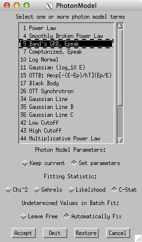
Before accepting the model, select the fitting statistic 'C-Stat', which is based upon the log-likelihood Cash statistic. Also, select the option 'Set Parameters', so that we have the option to input starting model parameters. Clicking 'Accept' brings up a dialog where the inputs can be changed. The fitting engine for RMFIT is quite robust and does not require bounds to be set for any parameter; the defaults here should be good enough, so select 'Accept'.
Two new windows appear; one window ('Fit Log') is where the detailed results of the spectral fit is displayed. They are reproduced below:
----------------------------------------------------------------------------------------------------

==> Dataset      : #0 INCLUDED

==> Data file    : /Users/trigger/bn080916009/glg_tte_n0_bn080916009_v00.fit

==> Response file: /Users/trigger/bn080916009/glg_cspec_n0_bn080916009_v04.rsp

==> Fit interval :  0.000: 70.656 s,  8.403000: 913.9359 keV, channels  4: 124


==> Fitting data...

==> MFIT F95 v1.7 2012 Sept. 7: Fit completed at Wed Jun 17 13:20:02 2015


TERM: Band's GRB, Epeak


        Amplitude    VARY      0.02251 +/-      0.00194 p/s-cm2-keV

        Epeak        VARY        294.8 +/-         40.4 keV

        alpha        VARY      -0.8525 +/-       0.0606

        beta         VARY       -1.947 +/-        0.165


==> Castor C-STAT = 261.86, DOF = 117

==> Photon Flux = 5.6665 +/- 0.10 ph/s-cm^2 in the interval: 10.00: 1000.0 keV

==> Energy Flux = 1.0825E-06 +/- 3.0E-08 erg/s-cm^2 in the interval: 10.00: 1000.0 keV


    The Normed Covariance Matrix = Correlation Coefficient Matrix:

   1.000 -0.964  0.945  0.539

  -0.964  1.000 -0.880 -0.684

   0.945 -0.880  1.000  0.450

   0.539 -0.684  0.450  1.000


    The global correlation coefficients of the varying parameters are:

   0.989  0.985  0.953  0.820
These results can be output to a text file for archiving purposes or added to a table of results that can be formatted for presentation by a wiki.
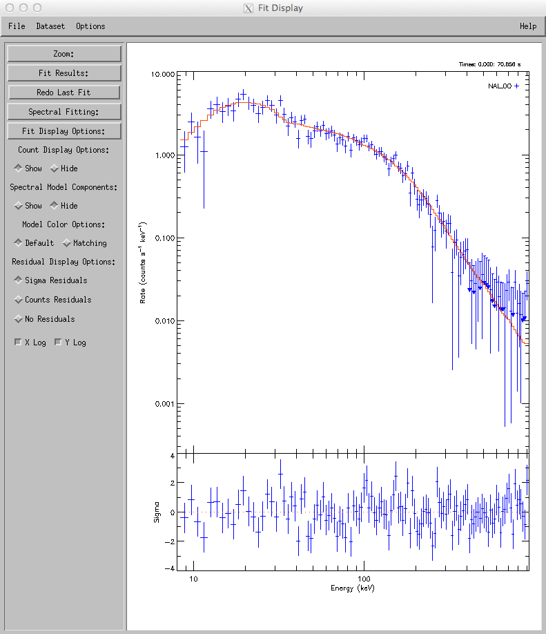
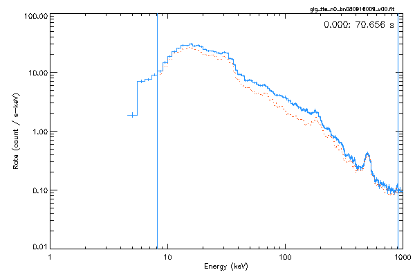
The 'Fit Display' is where the deconvolved spectrum is presented. The display menu items and options control the output in various ways. For instance, we can type 'n' (or select the menu item 'Fit Display Options:'->'Nu Fnu Spectrum') to display the unfolded spectrum as an E**2 f(E) plot. To just show the fitted function, select 'Hide' under 'Count Display Options' and 'No Residuals'. Of course, this is just the fitted function, evaluated with the best-fit paremeters and doesn't convey much useful information. Undoing these actions ('Show', 'Sigma Residuals' and 'c' for count rate spectrum), results in the figure shown (the color scheme has been customized to show black on white, with data from n0 in royal blue and the model histogram in orange; see the menu items under 'Options'->'Colors'). The plot can be archived as a '.png' formatted file by selecting the menu item 'File'->'Screenshot'.
Additional Notes:
- A much more comprehensive tutorial may be found at: Spectroscopy with RMFIT
- The analysis can be easily generalized to handle multiple GBM detectors, simply by loading more data files into RMFIT.
- The use of lookup files is strongly encouraged: previous spectral, source and background selections can be saved to a special (*.lu) file by the menu item 'File:'->'Lookup:'->'Save Lookup'. The next time the data file is loaded into RMFIT, the lookup file can automatically restore all selections. In addition, multiple data files can share the same selections by selecting the menu item 'File:'->'Lookup:'->'Read Lookup' and selecting the saved lookup. This is quite useful for fitting the same source intervals for multiple GBM NaI data fiels for the same burst.
- RMFIT can simultaneously analyze multiple data sets. In particular, it can accommodate joint LAT-GBM analysis of the LAT LLE data with GBM data.
- The user should be aware that the LAT photon data cannot be analyzed in RMFIT as-is.
Writing Out GBM PHA and BAK files for use with XSPEC:
rmfit uses PHA2 files i.e., fits files with multiple spectra. XSPEC uses PHA files i.e., files with a single spectrum, and expects a background file that is suitable for the spectrum provided by the user. Having chosen a suitable source region for a time-integrated spectral analysis, and having fit the background around this region, we will now save that information in a form that can be used in XSPEC. The files resulting from this analysis can be used in a joint GBM-LAT analysis.
(i) In the lightcurve window for n0, with your source region selected as 0.0:70.656 s, click the 'Misc' button along the top menu.
Select 'Background -> PHA' and use the default name. This saves a .BAK file for use in XSPEC.
It is very important to have saved your selections in a lookup file before the next step as you will be undoing your background selection.
(ii) Click 'Fit Background' and remove your background fit. To do this, click in the right margin of the plot to reset the intervals, then click in the left margin to accept a 'No background' selection.
(iii) Click the 'Misc' button along the top menu.
Select 'Selection -> PHA' and use the default name, which will end in .PHA. You will be warned that no background exists. This is ok as it is exactly what you want.
(iv) Read your background selection back in by using the 'File' button on the top menu. Select 'Lookup' then 'Read Lookup' and pick your saved information from the ensuing file list.
(v) Repeat steps (i) through (iv) for the other detectors you are using.
Last updated by: Rob Preece 06/17/2015