

Likelihood Tutorial
As is described in Cicerone (also see e.g. Abdo, A. A. et al. 2009, ApJS, 183, 46) the detection, flux determination and spectral modeling of Fermi LAT sources is accomplished by a maximum likelihood optimization technique. To illustrate how to use the Likelihood software, this narrative gives a step-by-step description for performing an unbinned likelihood analysis.
Unbinned vs Binned Likelihood
Unbinned likelihood analysis is the preferred method for spectral fitting of the LAT data (see Cicerone). However, a binned analysis is also provided for cases where the unbinned analysis cannot be used. For example, the memory required for the likelihood calculation scales with number of photons and number of sources. This memory usage becomes excessive for long observations of complex regions, necessitating the use of a binned analysis. To perform a binned likelihood analysis see the Binned Likelihood Tutorial.
Additional references:
- SciTools References
- Descriptions of available Spectral and Spatial Models
- Examples of XML Model Definitions for Likelihood
Prerequisites
You will need an event data file, a spacecraft data file (also referred to as the "pointing and livetime history" file), and the current isotropic emission model (available for download). You may choose to select your own data files, or to use the files provided within this tutorial. Custom data sets may be retrieved from the Lat Data Server.
Steps
- Make Subselections from the Event Data
Since there is computational overhead for each event associated with each diffuse component, it is useful to filter out any events that are not within the extraction region used for the analysis.
- Make Counts Maps from the Event Files
These simple FITS images let us inspect our data and help to pick out obvious candidate sources.
- Make an Exposure Map
This is needed for analyzing diffuse sources, and derived absolute fluxes.
- Download the latest model for the isotropic background
The latest model is isotropic_iem_v02.txt. All of the background models along with a description of the models are available here.
- Create a Source Model XML File
The source model XML file contains the various sources and their model parameters to be fit using the gtlike tool.
- Compute the Diffuse Source Responses
Skip step 6 unless you are using non-default background models.
Each event must have a separate response precomputed for each diffuse component in the source model.
- Run gtlike
Fitting the data to the model can give flux, errors, spectral index, and more.
- Make Test-Statistic Maps
These are used for point source localization and for finding weaker sources after the stronger sources have been modeled.
1. Make Subselections from the Event Data
For this case the original extraction of data from the first six months of the mission was done as described in the Extract LAT Data tutorial.
Selection of data:
- Search Center (RA, DEC) =(193.98, -5.82)
- Radius = 20 degrees
- Start Time (MET) = 239557417 seconds (2008-08-04 T15:43:37)
- Stop Time (MET) = 255398400 seconds (2008-02-04 T00:00:00)
- Minimum Energy = 100 MeV
- Maximum Energy = 100000 MeV
We provide the user with the two original event data files (file1 and file2) as well as with the spacecraft data file. In order to combine the two events files for your analysis, you must first generate a text file listing the events files to be included.
prompt> ls *_PH* > events.txt
This text file (events.txt) will be used in place of the input fits filename when running gtselect. The syntax requires that you use an @ before the filename to indicate that this is a text file input rather than a fits file.
When analyzing a point source, it is recommended that you include events with high probability of being photons. To do this, you should use gtselect to cut on the event class, keeping only event classes 3 and 4:
prompt> gtselect evclsmin=3 evclsmax=4
Be aware that evclsmin and evclsmax are hidden parameters. So to use them for a cut, you must type them in the command line.
We perform a selection to the data we want to analyze. For this example, we consider the diffuse class photons within a 20 degree region of interest (ROI) centered on the blazar 3C 279. We apply the gtselect tool to the data file as follows:
prompt> gtselect evclsmin=3 evclsmax=4

Input FT1 file[] @events.txt

Output FT1 file[] 3C279_events_filtered.fits

RA for new search center (degrees) (0:360) [] 193.98

Dec for new search center (degrees) (-90:90) [] -5.82

radius of new search region (degrees) (0:180) [] 20

start time (MET in s) (0:) [] 239557417

end time (MET in s) (0:) [] 255398400

lower energy limit (MeV) (0:) [] 100

upper energy limit (MeV) (0:) [] 100000

maximum zenith angle value (degrees) (0:180) [] 105

Done.

prompt>
In the last step we also selected the energy range and the maximum zenith angle value (105 degrees) as suggested in Cicerone. The Earth's limb is a stong source of background gamma rays. We filter them out with a zenith-angle cut. The value of 105 degrees is the one most commonly used. The filtered data are provided here.
After the data selection is made one must correctly calculate the exposure. There are several options for calculating livetime depending on your observation type and science goals. For a detailed discussion of these options, see Likelihood Livetime and Exposure in the Cicerone. To deal with the cut on zenith-angle in this analysis, we use the gtmktime tool to exclude the time intervals where the zenith cut intersects the ROI from the list of good time intervals (GTIs). This is especially needed if you are studying a narrow ROI (with a radius of less than 20 degrees), as your source of interest may come quite close to the Earth's limb. To make this correction you have to run gtmktime and answer "yes" at:
Apply ROI-based zenith angle cut[] yes
gtmktime also provides an opportunity to select GTIs by filtering on
information provided in the spacecraft file.
The current gtmktime filter expression recommended by the LAT team is:
DATA_QUAL==1 && LAT_CONFIG==1 && ABS(ROCK_ANGLE)<52.
This excludes time periods when some spacecraft event has affected the quality of the data, ensures
the LAT instrument was in normal science data-taking mode,and requires that the spacecraft be
within the range of rocking angles used during nominal sky-survey observations.
Here is an example of running gtmktime for our analysis of the region surrounding 3C 279.
prompt> gtmktime

Spacecraft data file[] spacecraft.fits

Filter expression[] (DATA_QUAL==1 && LAT_CONFIG==1 && ABS(ROCK_ANGLE)<52)

Apply ROI-based zenith angle cut[] yes

Event data file[] 3C279_events_filtered.fits

Output event file name[] 3C279_events_gti.fits
The data with all the cuts described above is provided in this link. A more detailed discussion of data selection can be found in the Data Preparation analysis thread.
To view the DSS keywords in a given extension of a data file, use the gtvcut tool and review the data cuts on the EVENTS extension. This provides a listing of the keywords reflecting each cut appplied to the data file and their values, including the entire list of GTIs.
prompt> gtvcut suppress_gtis=yes

Input FITS file[] 3C279_events_gti.fits

Extension name[EVENTS]

DSTYP1: POS(RA,DEC)

DSUNI1: deg

DSVAL1: CIRCLE(193.98,-5.82,20)


DSTYP2: TIME

DSUNI2: s

DSVAL2: TABLE

DSREF2: :GTI


GTIs: (suppressed)


DSTYP3: ENERGY

DSUNI3: MeV

DSVAL3: 100:100000


DSTYP4: EVENT_CLASS

DSUNI4: dimensionless

DSVAL4: 3:3


DSTYP5: ZENITH_ANGLE

DSUNI5: deg

DSVAL5: 0:105


prompt>
Here you can see the RA, Dec and ROI of the data selection, as well as the energy range in MeV, the event class selection, the zenith angle cut applied, and the fact that the time cuts to be used in the exposure calculation are definted by the GTI table.
Various science tools will be unable to run if you have multiple copies of a particular DSS keyword. This can happen if the position used in extracting the data from the data server is different than the position used with gtselect. It is wise to review the keywords for duplicates before proceeding. If you do have keyword duplication, it is advisable to regenerate the data file with consistent cuts.
2. Make Counts Maps from the Event Files
Next, we create a counts map of the region-of-interest (ROI), summed over photon energies, in order to identify candidate sources and to ensure that the field looks sensible as a simple sanity check. For creating the counts map, we will use the gtbin tool with the option "CMAP" as shown below:
prompt>  gtbin

This is gtbin version ScienceTools-v9r17p0-fssc-20100630

Type of output file (CCUBE|CMAP|LC|PHA1|PHA2) [] CMAP

Event data file name[] 3C279_events_gti.fits

Output file name[] 3C279_counts_map.fits

Spacecraft data file name[NONE]

Size of the X axis in pixels[] 160

Size of the Y axis in pixels[] 160

Image scale (in degrees/pixel)[] 0.25

Coordinate system (CEL - celestial, GAL -galactic) (CEL|GAL) [] CEL

First coordinate of image center in degrees (RA or galactic l)[] 193.98

Second coordinate of image center in degrees (DEC or galactic b)[] -5.82

Rotation angle of image axis, in degrees[] 0.0

Projection method e.g. AIT|ARC|CAR|GLS|MER|NCP|SIN|STG|TAN:[] AIT

prompt>  ds9 3C279_counts_map.fits &
The last command launches the visualization tool ds9 and produces this display:
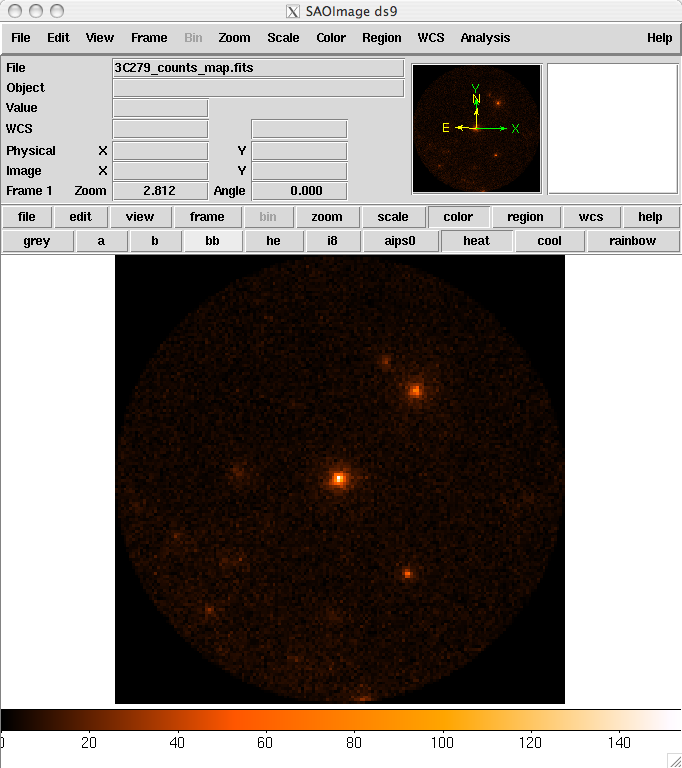
3C279_counts_map.fits
You can see two strong sources and several lesser sources in this map. Mousing over the positions of these two strong sources shows that they are likely 3C 279 and 3C 273, based on their positions. A more detailed discussion of data exploration can be found in the Explore LAT Data analysis thread.
3. Make an Exposure Map
We are now ready to create an exposure map. The type of exposure map used by Likelihood differs significantly from the usual notion of exposure maps, which are essentially integrals of effective area over time. The exposure calculation that Likelihood uses consists of an integral of the total response over the entire region-of-interest (ROI) data-space. See more information in the Cicerone.
Since the exposure calculation involves an integral over the ROI, separate exposure maps must be made for every distinct set of DSS cuts. This is important if, for example, one wants to subdivide an observation to look for secular flux variations from a particular source or sources. To view the DSS keywords in a given extension of a data file, use the gtvcut tool and review the data cuts for the EVENTS extension.
a. Generate Livetime Cubes
There are two tools needed for generating exposure maps. The first is gtltcube. This tool creates a livetime cube, which is a HealPix table, covering the full sky, of the integrated livetime as a function of inclination with respect to the LAT z-axis. For more information about the livetime cubes see the documentation in Cicerone.
Here is the example of how to run gtltcube:
prompt>  gtltcube

Event data file[] 3C279_events_gti.fits

Spacecraft data file[] spacecraft.fits

Output file[] 3C279_ltcube.fits

Step size in cos(theta) (0.:1.) [] 0.025

Pixel size (degrees)[] 1

Working on file spacecraft.fits

.....................!

prompt>
Note: Values such as "0.1" for "Step size in cos(theta)" are known to give unexpected results. Use "0.09" instead.
The livetime cube generated for this analysis can be found here.
Since gtltcube produces a FITS file covering the entire sky, the output of this tool could be used for generating exposure maps for regions-of-interest in other parts of the sky that have the same time interval selections. But use caution! The livetime cube MUST be regenerated if you change any part of the time interval selection. This can occur by changing the start or stop time of the events, or simply by changing the ROI selection or zenith angle cut (as these produce an ROI-dependent set of GTIs from gtmktime). See e.g. Data preparation in the Cicerone or the Data Preparation analysis thread.
Although the gtexpmap application (see below) can generate exposure maps for Likelihood without a livetime file, using one affords a substantial time savings.
b. Generate Exposure Maps
The tool gtexpmap creates an exposure map based on the event selection used on the input photon file and the livetime cube. The exposure map must be recalculated if the ROI, zenith, energy selection or the time interval selection of the events is changed. For more information about the exposure maps see the documentation in the Cicerone.
Creating the exposure map using the gtexpmap tool, we have:
prompt>  gtexpmap

The exposure maps generated by this tool are meant

to be used for *unbinned* likelihood analysis only.

Do not use them for binned analyses.

Event data file[] 3C279_events_gti.fits

Spacecraft data file[] spacecraft.fits

Exposure hypercube file[] 3C279_ltcube.fits

output file name[] 3C279_expmap.fits

Response functions[] P6_V3_DIFFUSE

Radius of the source region (in degrees)[] 30

Number of longitude points (2:1000) [] 120

Number of latitude points (2:1000) [] 120

Number of energies (2:100) [] 20

Computing the ExposureMap using 3C279_ltcube.fits

....................!

prompt>
Note that we have chosen a 30 degree radius "source region", while the acceptance cone radius specified for gtselect was 20 degrees. See discussion of region selection in Cicerone. This is necessary to ensure that events from sources outside the ROI are accounted for owing to the size of the instrument point-spread function. Half-degree pixels are a nominal choice; smaller pixels should result in a more accurate evaluation of the diffuse source fluxes but will also make the exposure map calculation itself lengthier. The number of energies specifies the number of logarithmically spaced intervals bounded by the energy range given in the DSS keywords. A general recommendation is 10 bins per decade. This is sufficient to accommodate the change in effective area with energy near 100 MeV.
Here is one image plane of the exposure map we just created:
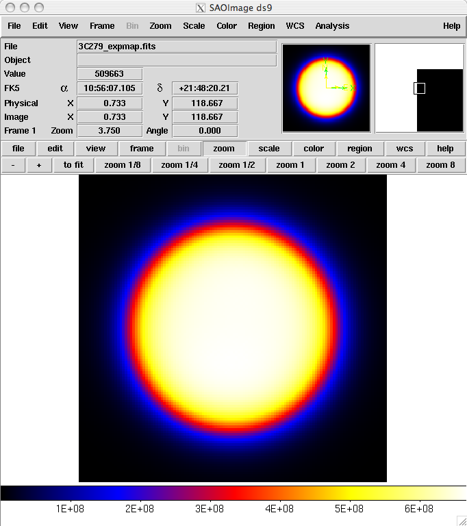
3C279_expmap.fits
4. Download the latest background models
When you use the lastest Galactic diffuse emission model, gll_iem_v02.fit, in a likelihood analysis you also want to use the corresponding model for the Extragalactic isotropic diffuse emission, which includes the residual cosmic-ray background. The latest isotropic model is isotropic_iem_v02.txt. For this example, you should save it in the same directory with your data. The isotropic spectrum is valid only for the P6_V3_DIFFUSE response functions and only for data sets with front + back events combined. All of the most up-to-date background models along with a description of the models are available here.
5. Create a Source Model XML File
The gtlike tool reads the source model from an XML file. The source model can be created using the model editor tool or by editing the file directly within a text editor. Review the help information for the model editor to learn how to run this tool.
Given the dearth of bright sources in the extraction region we have selected, our source model file will be fairly simple, comprising only the Galactic and Extragalactic diffuse emission, and point sources to represent the blazars 3C 279 and 3C 273. For this example, we use the diffuse background model as recommended by the LAT Team:
<?xml version="1.0" ?>

<source_library title="source library" xmlns="http://fermi.gsfc.nasa.gov/source_library">

<source name="EG_v02" type="DiffuseSource">

<spectrum file="./isotropic_iem_v02.txt" type="FileFunction">

<parameter free="1" max="1000" min="1e-05" name="Normalization"
scale="1" value="1" />

</spectrum>

<spatialModel type="ConstantValue">

<parameter free="0" max="10.0" min="0.0" name="Value" scale="1.0"
value="1.0"/>

</spatialModel>

</source>


<source name="GAL_v02" type="DiffuseSource">

<!-- diffuse source units are cm^-2 s^-1 MeV^-1 sr^-1 -->

<spectrum type="ConstantValue">

<parameter free="1" max="10.0"
min="0.0" name="Value" scale="1.0" value=
"1.0"/>

</spectrum>

<spatialModel file="$(FERMI_DIR)/refdata/fermi/galdiffuse/gll_iem_v02.fit" type="MapCubeFunction">

<parameter free="0" max="1000.0" min="0.001" name="Normalization" scale=
"1.0" value="1.0"/>

</spatialModel>


</source>

<source name="3C 273" type="PointSource">

<spectrum type="PowerLaw">

<parameter free="1" max="1000.0" min="0.001" name="Prefactor" scale="1e-09" value="10"/>

<parameter free="1" max="-1.0" min="-5.0" name="Index" scale="1.0" value="-2.1"/>

<parameter free="0" max="2000.0" min="30.0" name="Scale" scale="1.0" value="100.0"/>

</spectrum>

<spatialModel type="SkyDirFunction">

<parameter free="0" max="360" min="-360" name="RA" scale="1.0" value="187.25"/>

<parameter free="0" max="90" min="-90" name="DEC" scale="1.0" value="2.17"/>

</spatialModel>

</source>

<source name="3C 279" type="PointSource">

<spectrum type="PowerLaw">

<parameter free="1" max="1000.0" min="0.001" name="Prefactor" scale="1e-09" value="10"/>

<parameter free="1" max="-1.0" min="-5.0" name="Index" scale="1.0" value="-2"/>

<parameter free="0" max="2000.0" min="30.0" name="Scale" scale="1.0" value="100.0"/>

</spectrum>

<spatialModel type="SkyDirFunction">

<parameter free="0" max="360" min="-360" name="RA" scale="1.0" value="193.98"/>

<parameter free="0" max="90" min="-90" name="DEC" scale="1.0" value="-5.82"/>

</spatialModel>
</source>

</source_library>
The XML file used for this example is here. For more details on the available XML models, see:
- Descriptions of available Spectral and Spatial Models
- Examples of XML Model Definitions for Likelihood
6. Compute the Diffuse Source Responses
Skip this step if you are using the standard IRF (P6_V3_DIFFUSE) and diffuse background models distributed with the Science Tools. The diffuse response for the standard analysis has been precomputed and is included in the data file. However, if you are using a different IRF or diffuse model you MUST compute a custom diffuse response prior to continuing the analysis.
The gtdiffrsp tool uses the name in the xml model to identify the existence of calculated diffuse response values. This means that you need to use the provided diffuse files and match the naming scheme used for the diffuse components in the example above in order to take advantage of the precalculated diffuse response.
If these quantities are not precomputed using the gtdiffrsp tool, then gtlike will compute them at runtime. However, if multiple fits and/or sessions with the gtlike tool are anticipated, it is probably wise to precompute these quantities, as this step is very computationally intensive often taking ~hours to complete. The source model XML file must contain all of the diffuse sources to be fit. The gtdiffrsp tool will add columns to the event data file for each diffuse source. Here we have copied the events file to a new file (3C279_events_gti_altdiff.fits) that will be used to calculate the alternate/non-standard diffuse response.
prompt>  gtdiffrsp

Event data file[] 3C279_events_gti_altdiff.fits

Spacecraft data file[] spacecraft.fits

Source model file[] 3C279_input_model.xml

Response functions to use[] P6_V1_DIFFUSE

Working on...

3C279_events_gti_altdiff.fits.....................!

prompt>
This file would now be available for performing a likelihood analysis if you wished to use the P6_V1_DIFFUSE instrument response function (IRF). There are a number of IRFs distributed with the Fermi Science Tools. Some of these response functions, like P6_V3_DIFFUSE::FRONT, are designed to address only a subset of the events in the dataset, and thus would require you to make additional cuts before they could be used.
7. Run gtlike
We are now ready to run the gtlike application. You may need the results of the likelihood fit to be output in XML model form (e.g. to use in generating a test statistic map). To obtain an XML model output in addition to the standard results files, use the sfile parameter on the command line (as shown below) to designate the output XML model filename.
prompt>  gtlike refit=yes plot=yes sfile=3C279_output_model.xml

Statistic to use (BINNED|UNBINNED) [] UNBINNED

Spacecraft file[] spacecraft.fits

Event file[] 3C279_events_gti.fits

Unbinned exposure map[] 3C279_expmap.fits

Exposure hypercube file[] 3C279_ltcube.fits

Source model file[] 3C279_input_model.xml

Response functions to use[] P6_V3_DIFFUSE

Optimizer (DRMNFB|NEWMINUIT|MINUIT|DRMNGB|LBFGS) [] NEWMINUIT
Most of the entries prompted for are fairly obvious. In addition to the various XML and FITS files, the user is prompted for a choice of IRFs, the type of statistic to use, the optimizer, and some output file names.
The statistics available are:
- UNBINNED This is a standard unbinned analysis, described in this tutorial. If this option is chosen then parameters for the spacecraft file, event file, and exposure file must be given.
- BINNED See explanation in: Binned Likelihood Tutorial
There are five optimizers from which to choose: DRMNGB, DRMNFB, NEWMINUIT, MINUIT and LBFGS. Generally speaking, the faster way to find the parameters estimation is to use DRMNGB (or DRMNFB) approach to find initial values and then use MINUIT (or NEWMINUIT) to find more accurate results.
The application proceeds by reading in the spacecraft and event data, and if necessary, computing event responses for each diffuse source.
Here is the output from our fit:
Minuit did successfully converge.

# of function calls: 112

minimum function Value: 1033555.16329

minimum edm: 8.2613025e-05


(OMITTED MANY OUTPUTS HERE...)


Computing TS values for each source (4 total)

....!


3C 273:

Prefactor: 12.3809 +/- 0.50148

Index: -2.75107 +/- 0.0287348

Scale: 100

Npred: 3420.31

ROI distance: 10.4409

TS value: 5144.46


3C 279:

Prefactor: 9.60971 +/- 0.335547

Index: -2.30989 +/- 0.0192756

Scale: 100

Npred: 4449.21

ROI distance: 0

TS value: 9857.15


EG_v02:

Normalization: 1.03613 +/- 0.0185585

Npred: 40511.3


GAL_v02:

Value: 1.52101 +/- 0.0259699

Npred: 41474.7

WARNING: Fit may be bad in range [100, 199.526] (MeV)

WARNING: Fit may be bad in range [281.838, 562.341] (MeV)

WARNING: Fit may be bad in range [12589.3, 17782.8] (MeV)


Total number of observed counts: 89804

Total number of model events: 89855.5


-log(Likelihood): 1033555.179


Writing fitted model to 3C279_output_model.xml
Since we selected 'plot=yes' in the command line, a plot of the fitted data appears.
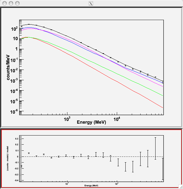
In the first plot the counts/MeV vs MeV are plotted. The points are the data, and the lines are the models. Error bars on the points represent sqrt(Nobs) in that band, where Nobs is the observed number of counts. The black line is the sum of the models for all sources. The colored lines follow the sources as follows:
- Black - summed model
- Red - first source in results.dat file (see below)
- Green - second source
- Blue - third source
- Magenta - fourth source
- Cyan - the fifth source
The second plot gives the residuals between your model and the data. Error bars here represent (sqrt(Nopbs))/Npred, where Npred is the predicted number of counts in each band based on the fitted model.
To assess the quality of the fit, look first for the words at the top of the output "<Optimizer> did successfully converge." Successful convergence is a minimum requirement for a good fit. Next, look at the energy ranges that are generating warnings of bad fits. If any of these ranges affect your source of interest, you may need to revise the source model and refit. You can also look at the residuals on the plot (bottom panel). If the residuals indicate a poor fit overall, you should consider changing your model file, perhaps by using a different source model definition, and refit the data.
If the fits and spectral shapes are good, but could be improved, you may wish to simply update your model file to hold some of the spectral parameters fixed. For example, by fixing the spectral model for 3C 273, you may get a better quality fit for 3C 279. Close the plot and you will be asked if you wish to refit the data.
Refit? [y]

n

Elapsed CPU time: 65.664521

prompt>
Here, hitting 'return' will instruct the application to fit again. We are happy with the result, so we type 'n' and end the fit.
Results
When it completes, gtlike generates two standard output files: results.dat with the results of the fit, and counts_spectra.fits with predicted counts for each source for each energy bin. The points in the plot above are the data points from the counts_spectra.fits file, while the colored lines follow the source model information in the results.dat file. If you re-run the tool in the same directory, these files will be overwritten by default. Use the clobber=no option on the command line to keep from overwriting the output files.
Interestingly, the fit details and the value for the -log(likelihood) are not recorded in the automatic output files. You should consider logging the output to a text file for your records.
In this example, we used the 'sfile' parameter to request that the model results be written to an output XML file, 3C279_output_model.xml. This file ontains the source model results that were written to results.dat at the completion of the fit.
Note: If you have specified an output XML model file and you wish to modify your model while waiting at the 'Refit? [y]' prompt, you will need to copy the results of the output model file to your input model before making those modifications.
The results of the likelihood analysis have to be scaled by the quantity called "scale" in the XML model in order to obtain the total photon flux (photons cm-2 s-1) of the source. You must refer to the model formula of your source for the interpretation of each parameter. In our example the 'prefactor' of our power law model of 3C273 has to be scaled by the factor 'scale'=10-9. For example the total flux of 3C273 is the integral between 100 MeV and 100000MeV of:
Prefactor x scale x (E /100)index=(12.3809x10-9 * (E/100)-2.75107
Errors reported with each value in the results.dat file are 1-sigma estimates (based on the inverse-Hessian at the optimum of the log-likelihood surface).
Other Useful Hidden Parameters
If you are scripting and wish to generate multiple output files without overwriting, the 'results' and 'specfile' parameters allow you to specify output filenames for the results.dat and counts_spectra.fits files respectively.
If you wish to include the effects of energy dispersion in your fit (the significance of this effect depends on each source), you can set the hidden parameter 'edisp=yes' in the command line.
If you do not specify a source model output file with the 'sfile' parameter, then the input model file will be overwritten with the latest fit. This is convenient as it allows the user to edit that file while the application is waiting at the 'Refit? [y]' prompt so that parameters can be adjusted and set free or fixed. This would be similar to the use of the "newpar", "freeze", and "thaw" commands in XSPEC.
8. Make Test-Statistic Maps
Ultimately, one would like to find sources near the detection limit of the instrument. The procedure used in the analysis of EGRET data was to model the strongest, most obvious sources (with some theoretical prejudice as to the true source positions, e.g., assuming that most variable high Galactic latitude sources are blazars which can be localized by radio, optical, or X-ray observations), and then create 'Test-statistic maps' to search for unmodeled point sources. These TS maps are created by moving a putative point source through a grid of locations on the sky and maximizing -log(likelihood) at each grid point, with the other, stronger, and presumably well-identified sources included in each fit. New, fainter sources are then identified at local maxima of the TS map.
The gttsmap tool can be run with or without an input source
model. However, for a useful visualization of the results of the fit, it is recommended you
use the output model file from gtlike. The file must be edited
so all parameters are fixed. Otherwise gttsmap will attempt a
refit of the entire model at every point on the grid. To see the field with the fitted sources
removed (i.e. a residuals map), fix all point source parameters before running the TS map.
To see the field with the fitted sources included, edit the model to remove all but the diffuse
components.
- For residuals map: 3C279_output_model_resid.xml
- For sources TS map: 3C279_output_model_diffonly.xml
Running gttsmap is extremely time-consuming, as the tool is performing a likelihood fit for all events at every pixel position. One way to reduce the time required for this step is to use very coarse binning and/or a very small region. In the following example, we run a TS map for the central 20x20 degree region of our data file, with .25 degree bins. This results in 6400 maximum likelihood calculations. The run time for each of the maps discussed below was approximately four days.
Here is an example of how to run the gttsmap tool to look for additional sources:
prompt>  gttsmap

Event data file[] 3C279_events_gti.fits

Spacecraft data file[] spacecraft.fits

Exposure map file[none] 3C279_expmap.fits

Exposure hypercube file[] 3C279_ltcube.fits

Source model file[] 3C279_output_model_resid.xml

TS map file name[] 3C279_tsmap_resid.fits

Response functions to use[] P6_V3_DIFFUSE

Optimizer (DRMNFB|NEWMINUIT|MINUIT|DRMNGB|LBFGS) [] NEWMINUIT

Fit tolerance[] 1e-5

Number of X axis pixels[] 80

Number of Y axis pixels[] 80

Image scale (in degrees/pixel)[] 0.25

Coordinate system (CEL|GAL) [] CEL

X-coordinate of image center in degrees (RA or l)[] 193.98

Y-coordinate of image center in degrees (Dec or b)[] -5.82

Projection method (AIT|ARC|CAR|GLS|MER|NCP|SIN|STG|TAN) [] AIT

.....................!
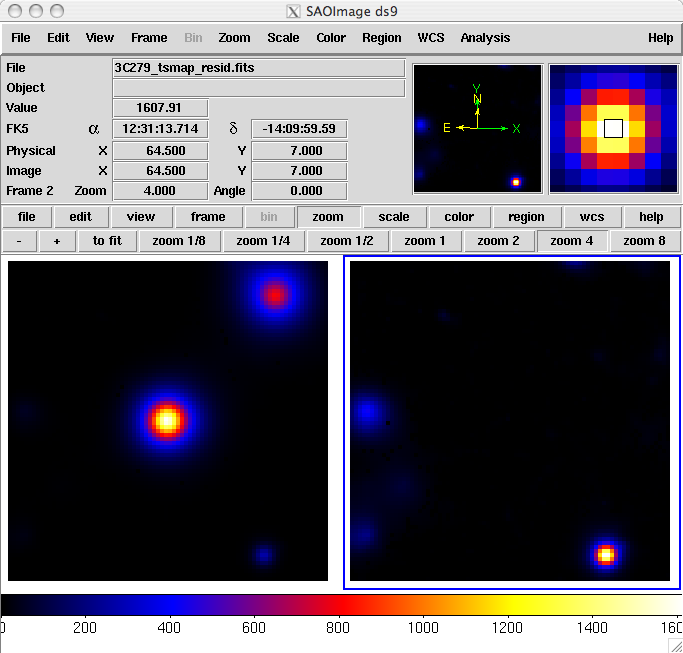
The output from the fit is below. Because generating TS maps takes a long time, you may wish to download the residuals and source files attached here. In the left panel, only diffuse sources were included in the analysis. The right panel shows the same field, but with the point souces (3C 279 and 3C 273) included in the model, and thus not included in the output image. This gives a pseudo-residuals map. The bright source clearly seen in the lower part of this image is a recently identified millisecond pulsar. The location of the cursor in the image indicates that this source had a TS of 1608 for the first six months of the mission.
In this example, the data set was small enough that an unbinned likelihood analysis is possible. With longer data sets, however, you may run into memory allocation errors, at which time it is necessary to move to binned analysis for your region. A typical memory allocation error looks like:
gtlike(10869) malloc: *** mmap(size=2097152) failed (error code=12)

*** error: can't allocate region

*** set a breakpoint in malloc_error_break to debug
If you encounter this error, then Binned Likelihood Analysis is for you!
Last updated by: Elizabeth Ferrara - 09/24/2010