Please Note: An updated, and maintained, version of this content is available on the Effective Area page.
Effective Area
The IRF sets in CALDB provide effective area separately for all event types: the front (thin) and back (thick) converters in the tracker, energy dispersion (edisp), and point spread function (psf). The key parameters that influence efficiency are the inclination angle (θ) and energy (E) of the incoming photon. The efficiency is given in discrete bins over this parameter space to fully encompass the range accessible to the LAT. The inclination angle is in 32 bins from cos(θ) = 0.2 to 1. The logarithm of the energy is in 64 bins from 5.62 MeV to 3.16 TeV (with 16 bins per decade below 17.8 GeV and 8 bins per decade above 17.8 GeV). The Fermitools perform an interpolation of the tabular efficiency to provide a smoothly varying efficiency for data analysis.
By default, the Fermitools do not take into account the phi dependence (phibins=0); however, this can be modified. The phi dependence has a larger variation on back converting events. (See section below on phi dependence.)
Examples from Pass 8 IRFs
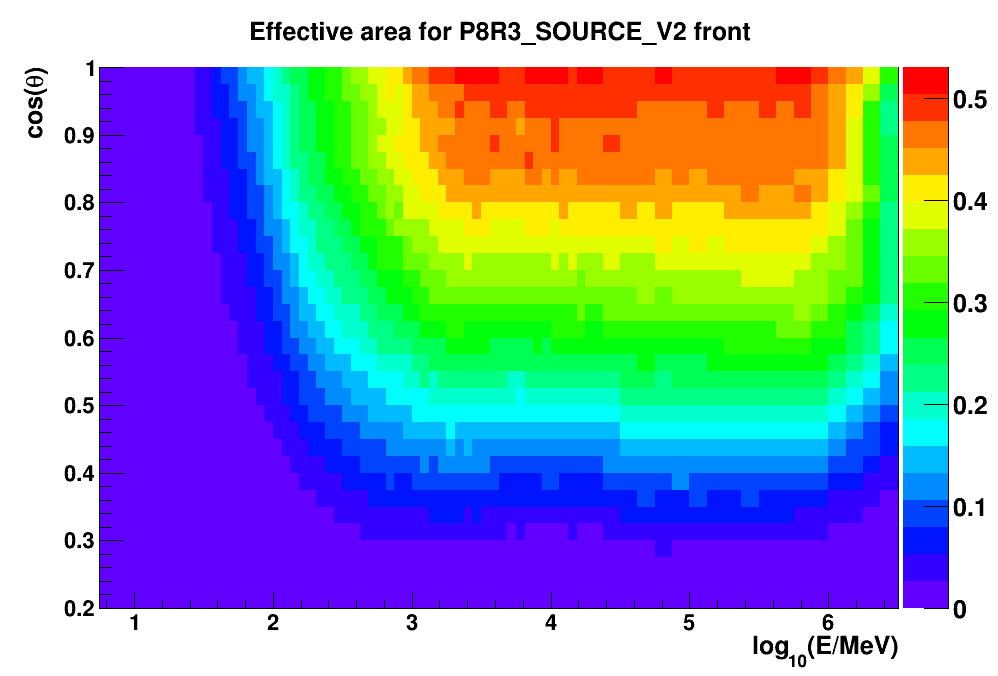
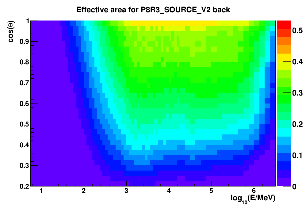
The plots below show the efficiency for the P8R3_SOURCE_V2 IRF set for both the Front (left) and Back (right) events. The color scale is in units of m2. Note the rapid change in efficiency with decreasing energy (and with increasing cosθ). This has some impact on the energy binning chosen for generating exposure maps used in spectral analysis of the LAT data.
| Front | Back |
|---|---|
 |
 |
Differences between IRF versions
The effective area description in the P8R2_SOURCE_V6 IRFs include these major improvements with respect to the previous P7REP_SOURCE_V15:
- The Pass 8 tracker pattern recognition reduces the fraction of mis-tracked events and provides an increase of the high-energy acceptance. In particular, photons converting in the lower part of the tracker (Back section) see an improvement in the off-axis effective area.
- Ghost signals away from the gamma-ray shower in Pass 8 are distinguished from the gamma-ray event in a clustering stage in the event reconstruction in the calorimeter. The recovered events contributed 5-10% to the improvement in the effective area.
- Utilizing the fast ACD signals provided to the LAT hardware trigger mitigate the impact of ghost signal in the slower ACD pulse-height measurements. This trigger information removes out-of-time signals from the ACD and increases the effective area.
Compared to the event selection corresponding to the previous P8R2_SOURCE_V6 IRFs, the one corresponding to P8R3_SOURCE_V2 has a few additional cuts that remove an anisotropic component of the residual background (mainly electrons), at the expense of a very minor loss (<1%) of acceptance.
Phi (φ) dependence of the effective area
The phi dependence of the effective area is not important for analyses integrating over long, or even moderate, time intervals (ex: results on the dependence on the exposure on 12-hour time scales is < 3% RMS at all energies). However, if the phi-dependence needs to be taken into account it should be included in any calculation that involves the effective area; for example, in gtexpcube2, gtexpmap, gtdiffrsp and gtsrcmaps. In addition, gtltcube needs to have the phibins option set in order for the phi-dependence to be accounted for in the gtexpmap and gtexpcube2 tools. In short, if gtltcube has the phibins option set, all subsequent tools that use the livetime cube will account for the phi-dependence. The number of energy bins over which the phi-dependence is characterized has been extended to cover 5.62 MeV to 3.16 TeV (23 bins in logE).
Particle background rate dependence of the effective area
One of the few surprises after launch regarding the performance of the LAT was the presence of 'ghost' events — signals in the subsystems from off-time or non-triggering events that are included with the readout from a triggered event. The issue is understandable if one considers the rates of background and the trigger latencies. However, the pre-launch event reconstruction was developed on clean, single-event Monte Carlo simulations. Noise in the subsystems was included, but not ghost tracks in the tracker or residual signals in the calorimeter. These ghost signals introduced an inefficiency in the event reconstruction — some perfectly good events were being misreconstructed and would fail classification cuts due to the ghosts. The effect of ghosts has now been partially mitigated with introduction of algorithms in Pass 8 to identify and remove ghost signals during the event reconstruction stage (see the discussion of Event Reconstruction in the Data Products page for more details). However inefficiencies due to ghost signals are still present at a lower level.
In order to account for ghosts, the LAT IRFs are generated with simulations that include real background events read out by the 2 Hz periodic trigger overlaid on the Monte Carlo events. Since the cosmic ray rate varies with the geomagnetic cutoff and the geomagnetic latitude varies markedly over the orbit of Fermi, the overlaid signals are sorted by geomagnetic latitude. The sample of ghost signals used in the simulations are chosen to match the rate of ghost events when the orbital conditions are averaged over a precession period.
For long integration periods the average correction is, to first order, a very good approximation. The inefficiency is energy dependent and is most important at low energies. On shorter timescales the rate-dependent inefficiency can depart from the orbit-averaged one. To account for these variations the LAT IRFs contain an additional correction to the effective area that depends on the livetime fraction.
The remarkably-linear dependence of the inefficiency on the background rate (or nearly equivalently, the deadtime fraction — the fraction of time the LAT is not accepting triggers because it is already reading out an event) and the independence of the inefficiency on inclination angle suggested a way to make detailed corrections for the inefficiency. Because the livetime (i.e., 1 minus the deadtime) was already included in the spacecraft files, the corrections were implemented in terms of livetime fraction (actually deadtime fraction). The livetime fraction is not strictly proportional to the rate of background particles incident on the LAT because not all events are read out, but it is an excellent proxy, with a scatter of less than 1%.
For analyses on short time scales (<<1 day) the average livetime fraction can be noticeably different from the overall average fraction. Also, for long integrations, the average rate-dependent inefficiency is not the same for all regions of the sky. The generally-higher rates near the South Atlantic Anomaly and the importance of times when the LAT is south of the equator to exposure of the southern sky mean that the average particle background are highest near the southern celestial pole.
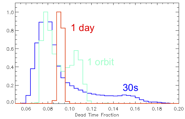
Here we can see how the average deadtime fraction varies on different timescales.
Starting with the Pass 7 and continuing with Pass 8, the IRFs extend the treatment of the estimation of background rates to account for these orbital variations in livetime. To summarize the procedure, the Monte Carlo with overlays were used to fit the ratio of effective areas as a linear function of livetime fraction (x) at the various energies.
![]()
By construction this must be equal to 1 when x is equal to the mean deadtime fraction (which is about 9%). Furthermore, p0 is the percent loss of efficiency per percent deadtime. It ranges from 3 at 100 MeV to close to 0 at 100 GeV.
We then performed a piecewise linear fit as a function of log10(Energy/MeV) to the parameters p0 and p1. Both parameters can be evaluated with the following piece of python code.
def p01(logE, a0, b0, a1, logEb1, a2, logEb2):

b1 = (a0 - a1)*logEb1 + b0

			b2 = (a1 - a2)*logEb2 + b1

			if logE < logEb1:

return a0*logE + b0

		    if logE < logEb2:

return a1*logE + b1

    		return a2*logE + b2
These constants (a0,b0,a1,logEb1,a2,logEb2) for both p0 and p1 are stored with the effective area fits files in the EFFICIENCY_PARAMS table, and are used to compute corrected livetime tables in gtltcube. (Note that in Pass 8 the format of the EFFICIENCY_PARAMS table has been modified to include only the parameters for the given IRF event type.)
Forward to Energy Dispersion
Back to the LAT PSF
Back to the beginning of the IRFs
Back to the beginning of the Cicerone