
Energy Dispersion
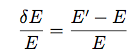
The energy dispersion of the LAT is defined in terms of the fractional difference between the reconstructed energy (E') and the true energy (E)of the events.
The energy resolution (i.e., the minimum 68% containment interval of the energy dispersion) is of order 10-15%, while the LAT energy band is over 4 orders of magnitude (30 MeV to over 300 GeV). Therefore, in many applications the energy dispersion can be neglected.
The default binning for the energy dispersion parameterization is 4 energy bins per decade, from 1.25 to 6.00 in log(Energy) (corresponding to the range 17.8 MeV to 1 TeV), and 8 angle bins, equally spaced from 0.2 to 1.0 in cos(θ). For each bin, a scaled energy dispersion is calculated, binned into a histogram, and then fitted as described below. First, we define
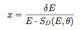
where the scaling factor depends on both true energy and true incidence angle:

All 6 parameters have distinct values for front and back events:
| c0 | c1 | c2 | c3 | c4 | c5 | |
|---|---|---|---|---|---|---|
| front | 0.0210 | 0.0580 | -0.207 | -0.213 | 0.042 | 0.564 |
| back | 0.0215 | 0.0507 | -0.220 | -0.243 | 0.065 | 0.584 |
The functional form of the analytical description of the LAT's Energy Dispersion Function is:
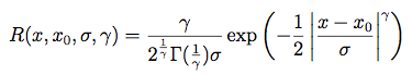
Note that this is normalized to 1 when integrated from -infinity to infinity. To account for the tails of the energy resolution, the IRFs use different exponents when the absolute value of  is larger than a characteristic value
  . Futhermore, given a noticeable left/right asymmetry, the curve is also parametrized separately left and right of the split point
  , so we have a total of four different ranges, and combined function is:
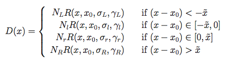
Note that the N are fixed by the requirements that the function be properly normalized and that it be continous at . In pratice the N are included in the fits file, but those values correspond to the arbitrary normalization of the fitting prodecure. The values for and the gammas are also stored in the FITS file, currently they are:
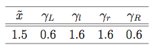
As an example, here is a histogram of the scaled deviation x, with the fitting function superimposed:
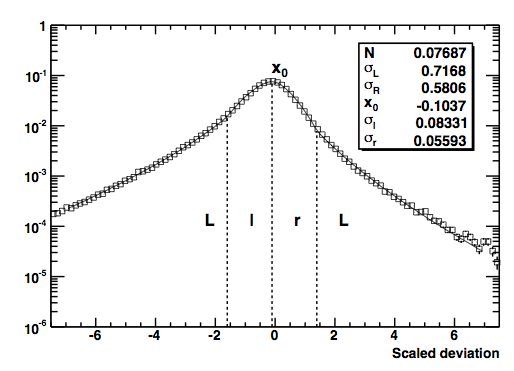
Finally, the and the sigmas are stored for each bin in log(E) and cos(theta) and comprise the bulk of the data in the energy dispersion fits files.
Note that by default the likelihood fitting tool gtlike does not include the energy dispersion in the fit. So long as the effective area is relatively flat (for example above 200 MeV) and you are not trying to resolve spectral features on a scale similar to the 6-15% energy resolution of the instrument, this causes a bias of at most 1-2% on the flux as a function of energy and similarly small biases on the spectral index and flux.
On the other hand, below about 100 MeV the effective area in P7REP_SOURCE_V15 does change fairly rapidly. Coupled with the energy dispersion this causes biases in the measured flux as a function of energy, and which depend on the spectral hardness of the source in question. Note that this effect was present at high energies (up to 200 MeV) when doing analysis with earlier "Pass 6" IRFs.
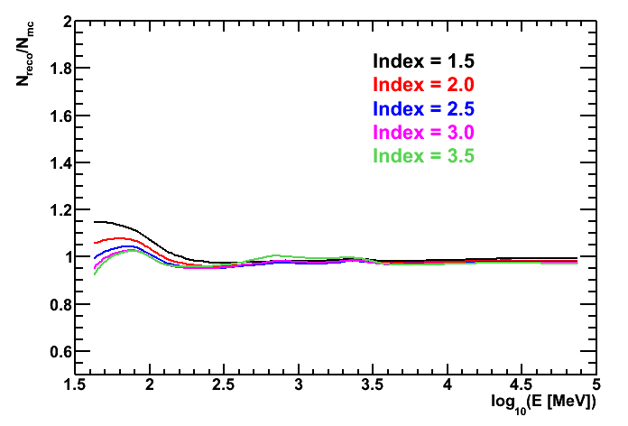
The bias on the flux as function of energy for several different spectral indices with the P7SOURCE_V6 IRFs. The bias for the P7REP_SOURCE_V15 is very similar.
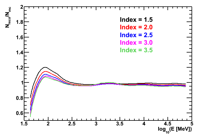
The bias on the flux as function of energy for the previous IRF set (P6_V11_DIFFUSE).
» Forward to LAT Sensitivity
» Back to Effective Area
» Back to the beginning of the IRFs
» Back to the beginning of the Cicerone

- Curator: J.D. Myers
- NASA Official: Elizabeth Hays
- Fermi FAQ, Comments, Feedback
- › Privacy Policy and Important Notices
- › Accessibility
- › Contact NASA
- › Page Last Updated: Wed, Sep 17, 2025