
Effective Area
The effective area describes the efficiency of the LAT for detecting gamma rays. The detector efficiency is derived from Monte Carlo simulations of gamma rays that are fully propagated though the instrument and event analysis from the physics interaction and electronics level to the trigger and filter algorithms and eventual event reconstruction and classification. See Atwood et al. 2009 for additional details of the simulation and instrument.
The IRF sets in CALDB provide effective area separately for the front (thin) and back (thick) converters in the tracker. The key parameters that influence efficiency are the inclination angle (θ) and energy (E) of the incoming photon. The efficiency is given in discrete bins over this parameter space to fully encompass the range accessible to the LAT. The inclination angle is in 32 bins from cos(θ) = 0.2 to 1. The logarithm of the energy is in 64 bins from 17.8 MeV to 1.78 TeV (with 16 bins per decade below 17.8 GeV and 8 bins per decade above 17.8 GeV). The Science Tools perform an interpolation of the tabular efficiency to provide a smoothly varying efficiency for data analysis.
Examples from Pass 7 IRFs
The plots below show the efficiency for the P7REP_SOURCE_V15 IRF set for both the Front (left) and Back (right) events. The color scale is in units of m**2. Note the rapid change in efficiency with decreasing energy (and with increasing cosθ). This has some impact on the energy binning chosen for generating exposure maps used in spectral analysis of the LAT data.
| Front | Back |
|---|---|
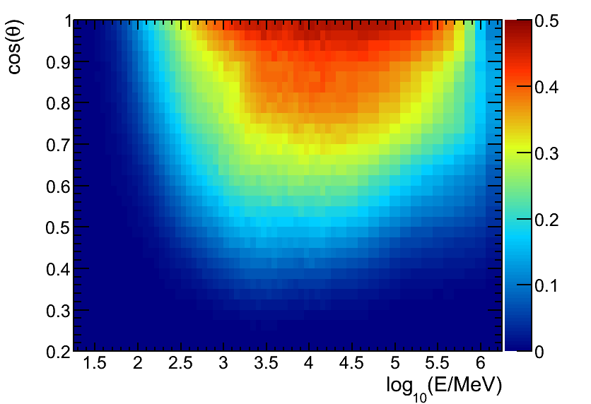 |
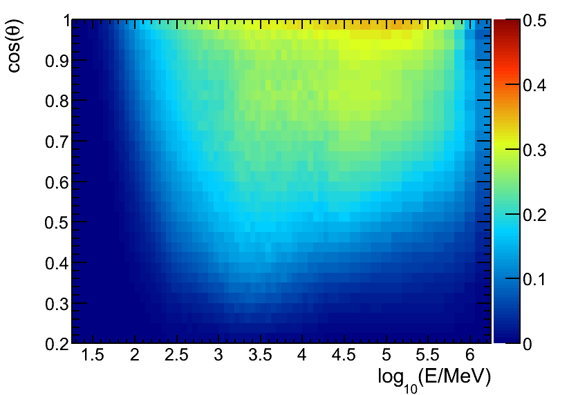 |
The P7REP_V15 IRFs account for inefficiencies caused by background events with signals in the detector that overlap in time with the gamma ray events (see "Post-launch performance of the Fermi Large Area Telescope").
The effective area does not account for instrument dead time (~8%) or scheduled inactivity during SAA passages (~13%). This correction is performed by the exposure calculation.
See the LAT performance page for additional plots and commentary.
Differences between IRF versions
The effective area description in the P7RPEP_V15 IRFs include two elements that were introduced in the early P6_V11 IRFs (and included in the P7_V6) IRFs but which were not included in the P6_V3 IRFs:
- A tabulation of the φ dependence of the effective area
- Extended treatment of efficiency losses induced by particle background pile-up to include variations with the orbital environment.
A third modification was made relative to the P7_V6 IRFs: the inclusion of a correction factor based on efficiency studies and consistency checks done with flight data. At low energies a mismatch between flight data and Monte Carlo was observed in the ratio of front-converting to back-converting events. The effective area tables have been modified to remove this discrepency while maintaining the same overall effective area. This correction and was less than 5% for all energies above 300 MeV, and less than 15% for all energies above 100 MeV.
Phi (φ) dependence of the effective area
Although the LAT is essentially symmetric with respect to reflections about 4 planes (X=0 (ie φ=0), X=Y (φ=45), Y=0 (φ=90) and X=-Y (φ=135) ), we have observed measurable differences in the effective area for photons coming in aligned with the sides (± X and Y axes) of the LAT relative to particles coming in along the corners (X = ± Y planes) of the LAT.
The LAT team has done studies which show that the effective area has a moderate φ dependence and that particular sources tend to be observed with a somewhat non-uniform φ coverage.
Both P6_V11 and P7_V6 IRFs include a table with the φ dependence in the effective area files. The main table still includes the average effective area. Parametrization of the φ dependency is done in 2 steps:
- Events, binned in MC energy and θ, are folded into a [0°-45°] φ range with the transformation
abs(abs(atan(McYDir/McXDir))*2./π-0.5)*2
- histograms obtained this way are fitted with a simple 2 parameter function:
"1 + [0]*x^[1]"
and the resulting fits parameters are stored in the φ-dependency fits table.
The RMS variation of the effective area as a function of φ is typically of the order of 5% and exceeds 10% only at low energies (less than 100 MeV) or far off-axis (θ > 60°) where the effective area is small, and at very high energies (> 100 GeV) where the event rate is small. This φ dependence of the effective area is not important for analyses integrating over long, or even moderate, time intervals.
Although the combined θ and φ dependence of the observing profile averages out only on year-long timescales, the eight-fold symmetry of the LAT combined with the rotation of the x-axis to track the Sun results in effective averaging over φ on short time scales. In fact, studies have found that ignoring the φ dependence of the effective area results in only a small variation of the exposure on 12-hour time scales (< 3% RMS at all energies).
Particle background rate dependence of the effective area
One of the few surprises after launch regarding the performance of the LAT was the presence of 'ghost' events — signals in the subsystems from off-time or non-triggering events that are included with the readout from a triggered event. The issue is understandable if one considers the rates of background and the trigger latencies. However, the pre-launch event reconstruction was developed on clean, single-event Monte Carlo simulations. Noise in the subsystems was included, but not ghost tracks in the tracker or residual signals in the calorimeter.
These ghost signals introduced an inefficiency in the event reconstruction - some perfectly good events were being misreconstructed and would fail classification cuts due to the ghosts. An extremely important advance for the high-level analysis was the development of the P6_V3 IRFs, which were generated from simulations that had actual ghost signals overlaid on the Monte Carlo events. The ghost signals were the contents of the 'events' read out by the 2 Hz periodic trigger. For the overlay they were sorted by geomagnetic latitude. The geomagnetic latitude varies markedly over the orbit and the corresponding variations in the geomagnetic cutoff result in large variations of the rate of cosmic rays incident on the LAT. P6_V3 IRFs were developed to have the overall average rate of ghost events and so have the average correction for rate-dependent inefficiency.
For long integration periods the average correction is to first order a very good approximation. The inefficiency is energy dependent and is most important at low energies.
The remarkably-linear dependence of the inefficiency on the background rate (or nearly equivalently the deadtime fraction — the fraction of time the LAT is not accepting triggers because it is already reading out an event) and the independence of the inefficiency on inclination angle suggested a way to make detailed corrections for the inefficiency. Because the livetime (i.e., 1 minus the deadtime) was already included in the FT2 files, the corrections were implemented in terms of livetime fraction (actually deadtime fraction). The livetime fraction is not strictly proportional to the rate of background particles incident on the LAT because not all events are read out, but it is an excellent proxy, with a scatter of less than 1%.
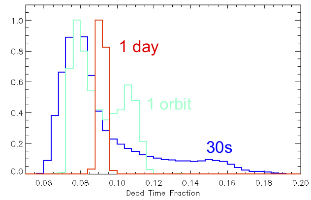
For analyses on short time scales (<<1 day) the average livetime fraction can be noticeably different from the overall average fraction. Also, for long integrations the average rate-dependent inefficiency is not the same for all regions of the sky. The generally-higher rates near the South Atlantic Anomaly and the importance of times when the LAT is south of the equator to exposure of the southern sky mean that the average particle background are highest near the southern celestial pole.
Here we can see how the average deadtime fraction varies on different timescales.
The Pass 7 IRFs extend the treatment of the estimation of background rates to account for these orbital variations in livetime. To summarize the procedure, the Monte Carlo with overlays were used to fit the ratio of effective areas as a linear function of livetime fraction (x) at the various energies.
η = Aeff(x) / Aeff(average) = p0x + p1
By construction this must be equal to 1 when x is equal to the mean deadtime fraction (which is about 9%). Furthermore, p0 is the percent loss of efficiency per percent deadtime. It ranges from 3 at 100 MeV to close to 0 at 100 GeV.
We then performed a piecewise linear fit as a function of log10(Energy/MeV) to the parameters p0 and p1. Both parameters can be evaluated with the following piece of python code.
def p01(logE, a0, b0, a1, logEb1, a2, logEb2):


b1 = (a0 - a1)*logEb1 + b0


			b2 = (a1 - a2)*logEb2 + b1


			if logE < logEb1:


				return a0*logE + b0


		    if logE < logEb2:


        		return a1*logE + b1


    		return a2*logE + b2
These constants (a0,b0,a1,logEb1,a2,logEb2) for both p0 and p1 and for both front and back type events are stored with the effective area fits files (in the EFFICIENCY_PARAMS table) and used to compute corrected livetime tables in gtltcube.
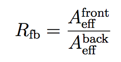
Correction of the Ratio of the Front to Back Effective Areas
The LAT team has seen a small but systematic discrepency between the ratio of front-converting to back-converting events observed in flight data to the Monte Carlo predictions. This discrepency is within the quoted systematic uncertainties, and results in relatively small (< 10%) biases in analyses such as the standard binned gtlike-based likelihood fittting that merges front- and back-converting events. However, when using either front- or back-only events, or when using the events seperatly in a combined fit, such as with unbinned gtlike-based likelihood fitting, this discrepency can lead to larger biases.
Accordingly, the LAT teams has used flight data to seperately correct the front and back effective area tables, while keeping the overall effective area unchanged.
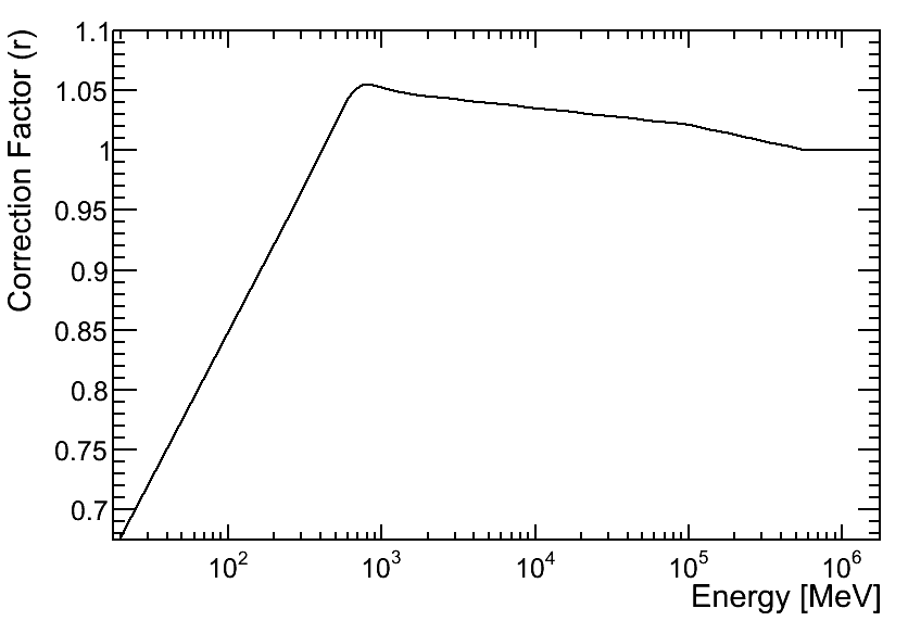
First, the LAT teams fit for the gamma-ray excess near the galactic plane as a function of energy seperately for front- and back-only events. They then compared the front-to-back ratio to the predicitions from exposure calculations to estimate an energy dependent correction factor, r.
Then they calculated the modified IRFs for each bin in logarithmic energy and cos(θ):
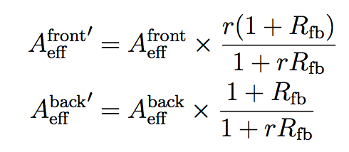
where the modified IRFs are primed and:
This formulation ensures that the total (front + back) effective area is unchanged, and that the angular dependence of the total effective area is unchanged. This LAT team made this choice because they could not determine if the front or the back effective area representation was more accurate.
The correction factor, r, is shown below and is less that 5% for all energies above 300 MeV, and less that 15% for all energies above 100 MeV.
» Forward to Energy Dispersion
» Back to the LAT PSF
» Back to the beginning of the IRFs
» Back to the beginning of the Cicerone

- Curator: J.D. Myers
- NASA Official: Elizabeth Hays
- Fermi FAQ, Comments, Feedback
- › Privacy Policy and Important Notices
- › Accessibility
- › Contact NASA
- › Page Last Updated: Wed, Sep 17, 2025