
Explore LAT Data (for Burst)
In this example we will examine the LAT data for a gamma-ray burst, based on the time and position derived from a GBM trigger. The steps outlined in this thread will allow you to get an idea of the general properties of this burst, but they are not sufficient for scientific analysis. (See the LAT GRB Analysis thread.)
Prerequisites
- gtbin
- gtselect
- gtvcut
- The FITS viewer fv
- The astronomical imaging and data visualization application ds9
Assumptions
It is assumed that:
- You are in your work directory.
- You know the time and location of the burst you wish to analyze.
Note: For the purposes of this thread, the relevant burst properties are:
- T0 = 00:12:45.614 UT, 16 September 2008, corresponding to 243216766.614 seconds (MET)
- Trigger # 243216766
- RA = 121.8 degrees
- Dec = -61.3 degrees
- You have extracted the files used in this tutorial; these files can be found here.
Steps
The analysis steps are:
- Extract the Data
- Data Selection
- Explore the Data
- Coordinates (J2000) = (121.8,-61.3)
- Search radius = 40 degrees
- Start time (MET) = 243216266.6 seconds (2008-09-16T00:04:26)
- Stop time (MET) = 243218766.6 seconds (2008-09-16T00:46:05)
- Energy range (MeV) = 30, 300000 MeV
- LAT data type = Extended
- Spacecraft data = "yes"
- The "evclass" that sets the event class selection, is a hidden parameter gtselect. By default, this parameter is set to "2", corresponding to "source" class events. For some aspects of the GRB analysis, we will want to use the lower quality photon selection, the "transient" class events. These cuts are optimized for transient sources for which the relevant timescales are sufficiently short that the additional residual charged particle backgrounds are much less significant. To obtain transient class events, the parameter has to be set to "0" at the command line. Refer to the Cicerone for a more detailed explanation about the event classification.
- A selection of INDEF indicates that the parameter's value will be read from the header of the input file; alternatively, we could have specified values within the acceptable ranges (the numbers in parentheses).
- As mentioned before, the LAT performance is optimized in the energy range (100 MeV, 300 GeV). This selection removes the low-energy, high-background events from the map.
- 40 degree acceptance cone cut centered on the GBM position
- GTIs corresponding to the out-of-SAA times in the spacecraft file, FT2.fits (in this case, the entire time interval is good)
- event class 0
- 100-300000 MeV energy cut
- zenith angle < 100 degrees
1. Extract the Data
Generally, one should refer to Extract LAT data tutorial, and use the time and spatial information from some source (here, the GCN notice #8245) to make the appropriate extraction cuts from the LAT data server. (The conversion between ISO 8601 date and MET can be performed using the HEASARC Time Conversion Utility).
We use the following parameters to extract the data from 500s before to 2000 seconds after the trigger time. This time range is selected to search for possible precursor and extended/afterglow emission in the LAT data:
2. Data Selection
a) Symlink the download filenames (optional)
After downloading the data, you should have two files with rather unwieldy names. We can symlink these to some shorter names and will use those names hereafter:
  prompt> ln -s L130911152323BD489E7F75_EV00.fits FT1.fits

  prompt> ln -s L130911152323BD489E7F75_SC00.fits FT2.fits
b) Filter out Earth limb emission
The FT1.fits file contains all of the photon data within 40 degrees of the GBM position in the time range that we have selected: (243216266.6, 243218766.6) MET. Many of these events will be Earth limb emission, which arise from cosmic ray interactions with the Earth's atmosphere. We can plot the measured zenith angle distribution of events in the FT1 file. Open the FT1 file in fv (more info on using this program can be found in the Explore LAT data section), select the "Hist" option for the EVENTS extension, and select ZENITH_ANGLE as the X column name:
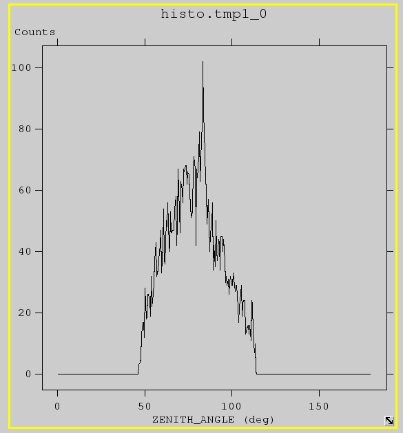
The burst shows up as the spike around 80 degrees. To filter out the Earth limb emission, we will apply a zenith angle cut of 100 deg using the gtselect tool:
  prompt> gtselect evclass=0

  Input FT1 file[] FT1.fits

  Output FT1 file[] filtered_zmax100.fits

  RA for new search center (degrees) (0:360) [INDEF]

  Dec for new search center (degrees) (-90:90) [INDEF]

  radius of new search region (degrees) (0:180) [INDEF]

  start time (MET in s) (0:) [INDEF]

  end time (MET in s) (0:) [INDEF]

  lower energy limit (MeV) (0:) [100]

  upper energy limit (MeV) (0:) [300000]

  maximum zenith angle value (degrees) (0:180) [180] 100

  Done.
Notes:
c) Review data cuts on photon data (optional)
At this point, it might be useful to review the cuts that have been applied to the data to be sure that the desired data selections are present. The effective data selections are stored in "data sub-space" keywords in the EVENTS header of the FT1 file. gtvcut can be used to display those selections (specify the hidden option suppress_gtis=no):
  prompt> gtvcut suppress_gtis=no

  Input FITS file[] filtered_zmax100.fits

  Extension name[EVENTS]

  DSTYP1: BIT_MASK(EVENT_CLASS,0,P7REP)

  DSUNI1: DIMENSIONLESS

  DSVAL1: 1:1


  DSTYP2: POS(RA,DEC)

  DSUNI2: deg

  DSVAL2: CIRCLE(121.8,-61.3,40)


  DSTYP3: TIME

  DSUNI3: s

  DSVAL3: TABLE

  DSREF3: :GTI


  GTIs:

  243216266.6  243218766.6


  DSTYP4: ENERGY

  DSUNI4: MeV

  DSVAL4: 100:300000


  DSTYP5: ZENITH_ANGLE

  DSUNI5: deg

  DSVAL5: 0:100
Here we see the cuts that were applied by the FSSC data server:
and the cuts we have applied using gtselect:
Note that we have not run gtmktime to correct the GTIs for these cuts. It is necessary to run gtmktime before performing an analysis that relies on the exposure. However, this step is not required to just take a quick look at the data.
3. Explore the Data
Counts maps
To get an idea of what the emission region looks like, we'll make a counts map of the region using the filtered data. For this, we use the gtbin tool:
prompt> gtbin

This is gtbin version ScienceTools-v9r32p5-fssc-20130826

Type of output file (CCUBE|CMAP|LC|PHA1|PHA2) [PHA2] CMAP

Event data file name[] filtered_zmax100.fits

Output file name[] cmap_zmax100.fits

Spacecraft data file name[NONE] FT2.fits

Size of the X axis in pixels[] 120

Size of the Y axis in pixels[] 120

Image scale (in degrees/pixel)[] 0.25

Coordinate system (CEL - celestial, GAL -galactic) (CEL|GAL) [CEL]

First coordinate of image center in degrees (RA or galactic l)[] 121.8

Second coordinate of image center in degrees (DEC or galactic b)[] -61.3

Rotation angle of image axis, in degrees[0.]

Projection method e.g. AIT|ARC|CAR|GLS|MER|NCP|SIN|STG|TAN:[AIT] STG
ds9 will allow us to view the counts map "cmap_zmax100.fits":
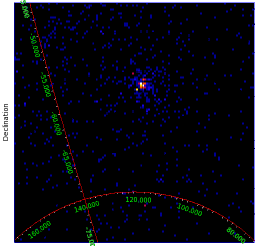
(Select "Coordinate Grid" under the "Analysis" menu, then "Coordinate Grid Parameters"; this counts map has "Publication" type black grids, with coordinates in degrees.)
Notes: the grid is centered on (121.8, -61.3), which was the original GBM position and the search center we have been using thus far. However, the burst is visible as a surplus of events around dec -56. For comparison, the official LAT position (from the LAT burst catalog) is (119.88, -56.59). By simply putting the mouse over the brightest pixel in the ds9 image, the RA and Dec of the likely burst location get displayed in the fk5 boxes (here, the new position is 119.5, -56.5). This is a quick method of localizing a burst, though not as accurate as fitting the data (described in the Likelihood Tutorial).
Light curves
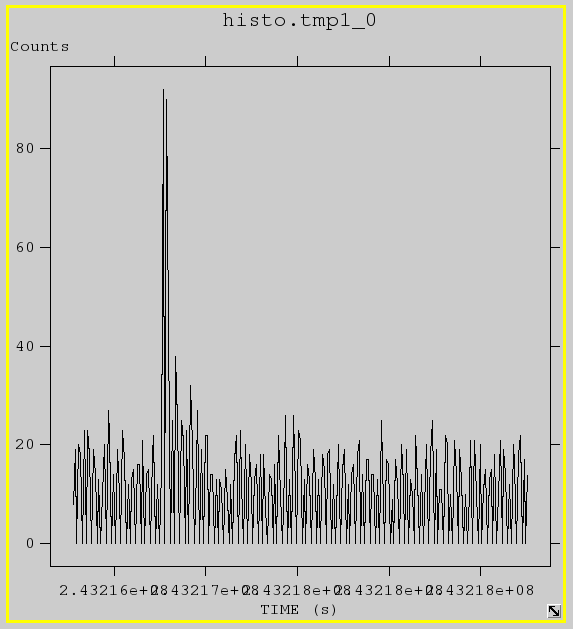
We can view a rough light curve in fv by creating a 1-D histogram of "TIME" over the entire length of the "filtered_zmax100.fits" file. After opening the file with fv, click on "Hist" button in the "EVENTS" extension. After selecting "TIME" as the column name for the "X" variable, to better view the light curve, we set the "Min" and "max" to be numbers at the start and stop time of our fits file (243216266.6 and 243218766.6) and the bin size to something reasonable (10 seconds in this example):
Now that we have a general idea of the prompt emission, we can use gtbin to create a counts light curve starting 50 seconds before the trigger and ending 100 seconds after:
prompt> gtbin

This is gtbin version ScienceTools-v9r32p5-fssc-20130826

Type of output file (CCUBE|CMAP|LC|PHA1|PHA2) [CMAP] LC

Event data file name[filtered_zmax100.fits]

Output file name[cmap_zmax100.fits] lc_zmax100.fits

Spacecraft data file name[FT2.fits]

Algorithm for defining time bins (FILE|LIN|SNR) [LIN]

Start value for first time bin in MET[0] 243216716.6

Stop value for last time bin in MET[0] 243216866.6

Width of linearly uniform time bins in seconds[0] 1
prompt> fv lc_zmax100.fits
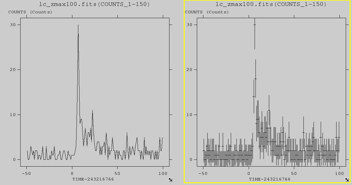
We have plotted the light curve with (right) and without errors (left). These were generated by selecting "Plot" in the "RATE" extension of the fits file. The x-value is TIME-243216766.6 (i.e., time minus trigger) and the y-value is COUNTS.
Note: Except for the period of the burst, almost all bins have 0-5 counts. This demonstrates that there is very little background for LAT observations of gamma-ray bursts.
More information on generating light curves and counts maps can be found in the Explore LAT data thread.
Last updated by: Davide Donato 08/31/2013

- Curator: J.D. Myers
- NASA Official: Elizabeth Hays
- Fermi FAQ, Comments, Feedback
- › Privacy Policy and Important Notices
- › Accessibility
- › Contact NASA
- › Page Last Updated: Wed, Sep 17, 2025