
GBM Data Extraction and Gamma-Ray Burst Analysis
This section provides the information needed to obtain the GBM data as well as a step-by-step example of extracting and modeling a GBM Gamma-Ray Burst observation and fitting the data using the X-Ray Spectral Fitting Package (Xspec).
Prerequisites
- gtbin
- gtbindef
- XSPEC, used as a spectral analysis tool in Step 3 of this procedure. (See Xanadu Data Analysis for X-Ray Astronomy.)
Assumptions
It is assumed that:
- You are in your work directory.
- T0 = 00:12:45.614 UT, 16 September 2008, corresponding to 243216766.614 seconds (MET)
- Trigger # 243216766
- RA = 121.8 degrees (= 08h 07m 12s)
- Dec = -61.3 degrees (= -61d 18m 00s)
- You have extracted the files used in this tutorial; these files can be found here. Alternatively, you could download the GBM data for 080916C as explained below.
- The approach illustrated in Section 2 and 3 assumes that the background is approximately constant through the burst duration and/or is negligible when compared to the burst emission. That is, this approximation is a valid in particular for bright and/or short burst. For analyzing GBM data, an alternative to XSPEC is RMFIT, a tool developed by the GBM team and available at the Fermi Science Support Center User Contributions page with an accompanying tutorial. RMFIT, which is GUI based and incorporates an interactive background fitting capability, and XSPEC can produce significantly different results and the user is strongly encouraged to compared the two methods in order to select the most accurate fit.
Note: For the purposes of this thread, the relevant burst properties are:
Steps:
1. Retrieve the GBM data
The GBM consists of 12 NaI detectors (8 keV to ~900 keV) and 2 BGO detectors (200 keV to ~40 MeV). Each detector views a different portion of the sky so that, for a particular burst, there will be varying amounts of signal in the different detectors. The data can be obtained from the HEASARC BROWSE GBM Burst Catalog (the column explanation can be retrieved at the help file page). There are multiple ways of easily locating a particular burst based solely on its name; e.g., for GRB080916C, we can:
- search for "bn080916*" as the trigger name. The wildcard character * is needed as the GBM naming convention includes the fraction of day as well as the date; in this case, GRB080916C corresponds to bn080916009.
- search for "GRB080916*" as the name. We want GRB080916009 for the purposes of this tutorial.
- search for "2008-09-16" as any of the times.
After obtaining the search results, click on "D" next to the burst in question (GRB080916009) for the data products. The Quicklook Plot is a set of light curves for all 12 NaI detectors.
The GBM burst data include files for all detectors, whether or not they were oriented to accumulate many counts from a burst. As a rule of thumb, we want to use the 2 or 3 NaI detectors with the brightest signals (the NaI detectors that triggered should have accumulated the most burst counts, although if FERMI slews to point towards a long burst, other detectors will record significant burst flux). More detectors can be used, but for the most part, they will not increase the significance of the fits.
For this burst, we will choose NaI0 (which triggered), NaI3, and NaI4. Because we have chosen detectors between 0 and 5, we also select BGO0. If we had chosen NaI detectors 6-11, we would use BGO1. If both low- and high-numbered NaI are being used, then select both BGO detectors. More specific lightcurves can be found in the quicklook products directory.
In the page where the above set of light curves is located, you can select the "GBM Trigger Products (current)" directory to retrieve the full data for the all the detectors. They are sometimes updated to newer versions, indicated by the v0# numbers at the end of the file name (the version numbers are unimportant, and do not need to be consistent across the different files). The files for the NaI and BGO detectors are labelled differently: The corresponding files for the NaI detectors have n# (n0 to n9, na, or nb, with the last two corresponding to detectors #10 and #11) while for the BGO detectors BGO have b0 or b1. The naming convention for the GBM files can be found in the GBM Data Products page and in the Cicerone (See Data - GBM Data Products).
Instead of checking the above set of light curves, another way to select the triggered detector is from the burst data files. For example, look for the 'DET_MASK' keyword in the primary header of the file that begins "glg_trigdat" (use the FTOOLS fkeyprint to display the content of the keyword). This keyword provides a string that indicates which detectors triggered: the label "1" or "0" denotes if the NaI detector were triggered or not. Therefore, the string '000110000000' for 080916C means that NaI detectors 3 and 4 only were actually triggered.
For GRB080916C, the relevant files for the NaI detectors are:
- glg_cspec_n#_bn080916009_v0#.pha: The CSPEC spectral file (PHA2) for the GRB, binned into 1.024s time bins and 128 energy channels.
- glg_cspec_n#_bn080916009_v0#.fit: The TTE (time-tagged event) data file for individual photons, binned into 128 energy channels.
- glg_cspec_n#_bn080916009_v0#.rsp: The instrument response file for each detector. These are used for both CSPEC and TTE data.
- glg_cspec_n#_bn080916009_v0#.bak: The CSPEC spectral file (PHA2) for the background.
TTE files only cover ~300 s of data around the trigger time, and take longer to process. CSPEC files cover a longer time interval, and are good for longer events where the TTE files might not be sufficient for background fitting. The GBM team will update files as better data products become available. For example, response files may be updated as better burst positions become available (e.g., because Swift or the IPN provide a more accurate position that the GBM position).
In this tutorial, we will be analyzing the TTE data for NaI0. We will need the .fit file and the .rsp file, as well as the header file "glg_tcat_all_bn080916009_v02.fit".
2. Creating and viewing lightcurves
The TTE file contains information for each individual photon. We use gtbin to create a lightcurve:
prompt> gtbin


This is gtbin version ScienceTools-v9r23p1-fssc-20111006


Type of output file (CCUBE|CMAP|LC|PHA1|PHA2) [PHA2] LC


Event data file name[] glg_tte_n0_bn080916009_v01.fit


Output file name[] glg_tte_n0_bn080916009_v01.lc


Spacecraft data file name[NONE]


Algorithm for defining time bins (FILE|LIN|SNR) [LIN]


Start value for first time bin in MET[] 243216746


Stop value for last time bin in MET[] 243217066


Width of linearly uniform time bins in MET[] 0.25
Notes:
- The choice of LC for 'Type of output file' indicates that you want to create a lightcurve.
- The choice of LIN for 'Algorithm for defining time bins' indicates that you want a linear time grid. The width of the time bins is the last parameter entered.
- The start and stop times are in Mission Elapsed Time. If you type INDEF the program takes the tstart and tstop of the original event.
Next we plot the lightcurve in fv, shifted so that the trigger time is at t=0:
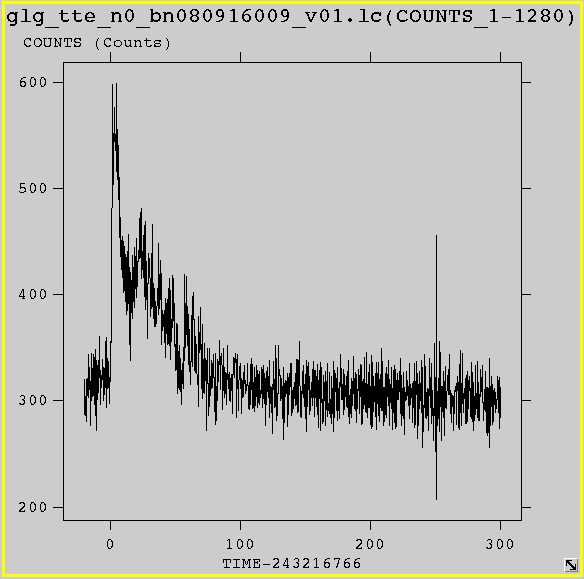
Select the "PLOT" option for the "RATE" extension of the .lc file; plot "TIME-243216766.614" as the x value and "COUNTS" as the y-value. Plotting lightcurves as counts vs FERMI's natural time system (i.e., MET) usually results in an x-axis that is not very informative because of the large difference in scale between burst durations (10's of seconds) and MET. Therefore it is useful to plot lightcurves as counts vs. time relative to the trigger time. a quantity that is provided in the HEASARC BROWSE GBM Burst Catalog, but is also found in the primary header of the GBM burst data files as the keyword 'TRIGTIME'.
The time unit in the FERMI data files is Mission Elapsed Time (MET), the number of seconds since midnight January 1, 2001 (UTC), as is described in the Cicerone. (See Data - Time in FERMI Data Analysis.). The xTime Date/Time Conversion Utility converts between FERMI's MET and other time systems.
It looks like the burst lasted for about 70 seconds for this detector; we'll use this as a time cut in order to construct a spectrum. We first create an ascii file defining our time cuts, which we will call "timeBins.txt":
243216736 243216756


243216766 243216836
The first line contains 20s of pre-burst background data, which can be used for spectral analysis; the second line is the approximate MET time range for the burst. Next we run gtbindef:
prompt> gtbindef


This is gtbindef version ScienceTools-v9r23p1-fssc-20111006


Type of bins, E -- energy or T -- time[E] T


File containing the ascii bin definitions[] timeBins.txt


Output file name[] timeBins.fits
We use gtbin to create a PHA2 file (a PHA file which contains an energy spectrum for each time bin), using the file we have just created to define our time bins:
Note: gtbin currently has a bug when making pha2 files; it requires the parameters tstart and tstop to have values set, even though they are not used when time bins are specified in a file. Although the actual values tstart and tstop values should not matter, as long as tstop > tstart, it is recommended to use values well outside the actual time range. You can specify these values on the command line:
prompt> gtbin tstart=243216500 tstop=243217500


This is gtbin version ScienceTools-v9r23p1-fssc-20111006


Type of output file (CCUBE|CMAP|LC|PHA1|PHA2) [LC] PHA2


Event data file name[glg_tte_n0_bn080916009_v01.fit]


Output file name[glg_tte_n0_bn080916009.lc] glg_tte_n0_bn080916009.pha


Spacecraft data file name[NONE]


Algorithm for defining time bins (FILE|LIN|SNR) [LIN] FILE


Name of the file containing the time bin definition[NONE] timeBins.fits
Now this PHA2 spectral file, along with the corresponding response matrix file ("glg_cspec_n0_bn080916009_v07.rsp"), can be analyized with XSPEC.
3. XSPEC analysis
What follows is a simple analysis of the NaI #0 detector spectrum of GRB080916C using Xspec. For more detailed examples, consult the XSPEC manual.
1. Start XSPEC
Note: The default version is now release 12 (XSPEC12).
2. Load in the data:
XSPEC12> data glg_tte_n0_bn080916009.pha{2}


1 spectrum  in use


Spectral Data File: glg_tte_n0_bn080916009.pha{2}  Spectrum 1


Net count rate (cts/s) for Spectrum:1  1.609e+03 +/- 4.806e+00


 Assigned to Data Group 1 and Plot Group 1


  Noticed Channels:  1-128


  Telescope: GLAST Instrument: GBM  Channel Type: PHA


  Exposure Time: 69.65 sec


 Using fit statistic: chi


 No response loaded.


***Warning!  One or more spectra are missing responses,


               and are not suitable for fit.
Recall that we specified two bins: 1) background, and 2) burst, each with its own energy spectrum. The data come from our second bin, so that we specify 2 in brackets when we load in the data. Because the response matrix was not specified in the header of the spectral file, it has not been automatically loaded and a warning has been printed out. Load in the response matrix:
3. Load the response file:
XSPEC12> resp glg_cspec_n0_bn080916009_v07.rsp


***Warning: No TLMIN keyword value for response matrix FCHAN column.


            Will assume TLMIN = 1.


Response successfully loaded.
4. Load in the background (the first time bin):
XSPEC12> back glg_tte_n0_bn080916009.pha{1}


Net count rate (cts/s) for Spectrum:1  3.460e+02 +/- 1.029e+01 (21.5 % total)
Most binned spectra have high and low energy channels, that are beyond the instrument response function's believable energy range, are affected by non-linearities, or are overflow channels (all counts above a certain energy end up in that channel). These channels should not be included in fitting spectra; in XSPEC terminology these channels are 'ignored.' Assuming that the GBM channels run from 1 to 128 the following channels should always be ignored:
- NaI spectra—all channels below 8 keV, and then channel 128. Note that 8 keV corresponds to different channels in different NaI detectors, and therefore the low energy channels that should be ignored will vary from detector to detector
- BGO spectra—channels 1 and 128
These are conservative ranges (i.e., ignoring as few channels as possible) and more realistically it will be necesary to ignore a few additional channels on either end. If you find that the residual (fit minus actual count numbers) for a few channels at either end of the fitted spectrum are particularly large, then these channels are probably affected by systematics and should be ignored.
5. In our case, we ignore a large number of channel:
XSPEC12> ign 1-5,100-**


     5 channels (1,5) ignored in spectrum #     1


    29 channels (100,128) ignored in spectrum #     1
6. Next, we load a model. The "grb" or "grbm" model is the Band function:
XSPEC12> mo grb


Input parameter value, delta, min, bot, top, and max values for ...


             -1       0.01(      0.01)        -10         -3          2          5


1:grbm:alpha>


             -2       0.01(      0.02)        -10         -5          2         10


2:grbm:beta>


            300         10(         3)         10         50       1000      10000


3:grbm:tem>


              1       0.01(      0.01)          0          0      1e+24      1e+24


4:grbm:norm>


========================================================================


Model grbm<1> Source No.: 1   Active/On


Model Model Component  Parameter  Unit     Value


 par  comp


   1    1   grbm       alpha               -1.00000     +/-  0.0


   2    1   grbm       beta                -2.00000     +/-  0.0


   3    1   grbm       tem        keV      300.000      +/-  0.0


   4    1   grbm       norm                1.00000      +/-  0.0


________________________________________________________________________


 Chi-Squared =   3.844704e+06 using 94 PHA bins.


 Reduced chi-squared =       42718.93 for     90 degrees of freedom


 Null hypothesis probability =   0.000000e+00


 Current data and model not fit yet.
7. Fit the data:
XSPEC12> fit


<...skip output...>


========================================================================


Model grbm<1> Source No.: 1   Active/On


Model Model Component  Parameter  Unit     Value


 par  comp


   1    1   grbm       alpha               -1.00785     +/-  0.132980


   2    1   grbm       beta                -3.06796     +/-  0.843127


   3    1   grbm       tem        keV      416.990      +/-  168.483


   4    1   grbm       norm                1.77511E-02  +/-  3.97780E-03


________________________________________________________________________


 Chi-Squared =         99.91 using 94 PHA bins.


 Reduced chi-squared =         1.110 for     90 degrees of freedom


 Null hypothesis probability =   2.228741e-01
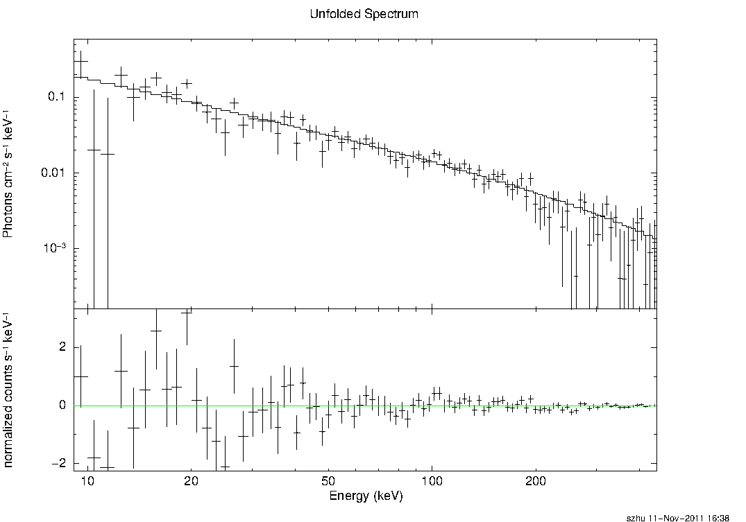
8. Plot the results:
XSPEC12> cpd /xs


XSPEC12> setplot energy


XSPEC12> plot ldata res


XSPEC12> plot uf res
Notes:
- The cpd command defines the graphics device, here xserve.
- The setplot command changes the x axis from channels to energy.
- The plot command indicates that the data and model should be plotted in logarithmic scales and showing the residuals.
- "uf" indicates that we want to plot the unfolded spectrum.
The figure below shows the spectrum obtained for this example.
Additional Notes:
- The XSPEC analysis can be easily generalized to handle multiple GBM detectors, using the data grouping capabiliy of XSPEC.
- XSPEC can simultaneously analyze multiple data sets. In particular, it can accommodate joint LAT-GBM analysis (see the combined LAT-GBM analysis page).
- As it is mentioned in the » Assumptions section, RMFIT can be used to analyze the GBM data, although the user should be aware that the LAT data cannot be analyzed in RMFIT as-is, that is, only the method explained above can generate the files to perform the combined LAT/GBM analysis.
Last updated by: Elizabeth Ferrara 08/07/2012

- Curator: J.D. Myers
- NASA Official: Elizabeth Hays
- Fermi FAQ, Comments, Feedback
- › Privacy Policy and Important Notices
- › Accessibility
- › Contact NASA
- › Page Last Updated: Thu, Oct 11, 2018