Data

+ System Overview
+ Software Download
+ Documentation
+ Cicerone
+ Analysis Threads
+ User Contributions

Extended Source Analysis

The analysis of an extended source is performed similarly to the process described in the binned likelihood tutorial. The only extra step needed is to create a two dimensional template that describes the object you are wanting to analyze. This template can be created from several different sources including maps from other observatories or you can create your own from scratch. There are a few simple rules you have to follow in creating your template but once you've done that, pretty much any shape is possible to model.

This sample analysis is based on the Centaurus A analysis performed by the LAT team and described in Abdo, A. A. et al. 2010, Science, 328, 728. At certain points we will refer to this article and its suplement as well as the Cicerone. The goal of this tutorial is to reproduce the data analysis performed in this publication including calculating the spectral shape and fluxes of the central core of Cen A and the large radio lobes. This tutorial uses a user contributed tool (make2FGLxml) and assumes you have the most recent ScienceTools installed. We will also make significant use of python, so you might want to familiarize yourself with python (there's a beginner's guide at http://wiki.python.org/moin/BeginnersGuide). This tutorial also assumes that you've gone through the non-python based binned likelihood thread. It is also useful if you have gone through the Likelihood Analysis with Python tutorial. This tutorial should take approximately 8 hours to complete (depending on your computer's speed) if you do everything but there are some steps you can skip along the way which shaves off about 4 hours of that.

Note: In this tutorial, commands that start with '[user@localhost]$' are to be executed within a shell environment (bash, c-shell etc.) while commands that start with '>>>' are to be executed within an interactive python environment. Commands are in bold and outputs are in normal font. Text in ITALICS within the boxes are comments from the author.

Get the Data

For this thread the original data were extracted from the LAT data server with the following selections (these selections are similar to those in the paper):

Search Center (RA,Dec) = (201.47,-42.97)
Radius = 30 degrees
Start Time (MET) = 239557420 seconds (2008-08-04T15:43:40)
Stop Time (MET) = 265507200 seconds (2009-06-01T00:00:00)
Minimum Energy = 210 MeV
Maximum Energy = 31000 MeV

We've provided direct links to the event files as well as the spacecraft data file if you don't want to take the time to use the download server. For more information on how to download LAT data please see the Extract LAT Data tutorial.

You'll first need to make a file list with the names of your input event files:


[user@localhost]$ ls -1 *PH*.fits > CenA.list

In the following analysis we've assumed that you've named your list of data files CenA_events.list and the spacecraft file SC.fits.

Perform Event Selections

We are going to follow the prescription described in the unbinned likelihood tutorial to filter and prepare our data set.

First, execute gtselect:


[user@localhost]$ gtselect evclass=2
 
Input FT1 file[] @CenA.list

Output FT1 file[] CenA_filtered.fits

RA for new search center (degrees) (0:360) [] 201.47

Dec for new search center (degrees) (-90:90) [] -42.97

radius of new search region (degrees) (0:180) [] 10

start time (MET in s) (0:) [] 239557420

end time (MET in s) (0:) [] 265507200

lower energy limit (MeV) (0:) [] 210

upper energy limit (MeV) (0:) [] 31000

maximum zenith angle value (degrees) (0:180) [] 100

Done.

Next, you need to run gtmktime with a similar filter as that used in the publication.


[user@localhost]$ gtmktime 

Spacecraft data file[] SC.fits 

Filter expression[](DATA_QUAL>0)&&(LAT_CONFIG==1)

Apply ROI-based zenith angle cut[] yes

Event data file[] CenA_filtered.fits 

Output event file name[] CenA_filtered_gti.fits

Create and View a Counts Map

Now we can go ahead and create a counts map of the region so we can visualize the lobes and see the core of CenA in gamma rays. We can't make any quantitative statements yet since we haven't produced a template to model but we can at least look and see what we have.


[user@localhost]$ gtbin

This is gtbin version ScienceTools-v9-27-01

Type of output file (CCUBE|CMAP|LC|PHA1|PHA2) [] CMAP

Event data file name[] CenA_filtered_gti.fits 

Output file name[] CenA_CMAP.fits

Spacecraft data file name[] NONE

Size of the X axis in pixels[] 140

Size of the Y axis in pixels[] 140

Image scale (in degrees/pixel)[] 0.1

Coordinate system (CEL - celestial, GAL -galactic) (CEL|GAL) [] CEL

First coordinate of image center in degrees (RA or galactic l)[] 201.47

Second coordinate of image center in degrees (DEC or galactic b)[] -42.97

Rotation angle of image axis, in degrees[] 0

Projection method e.g. AIT|ARC|CAR|GLS|MER|NCP|SIN|STG|TAN:[] AIT

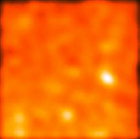
Open this FITS image up in your favorite FITS viewer such as ds9. If you use the default settings you'll see the following (using the 'heat' color map):

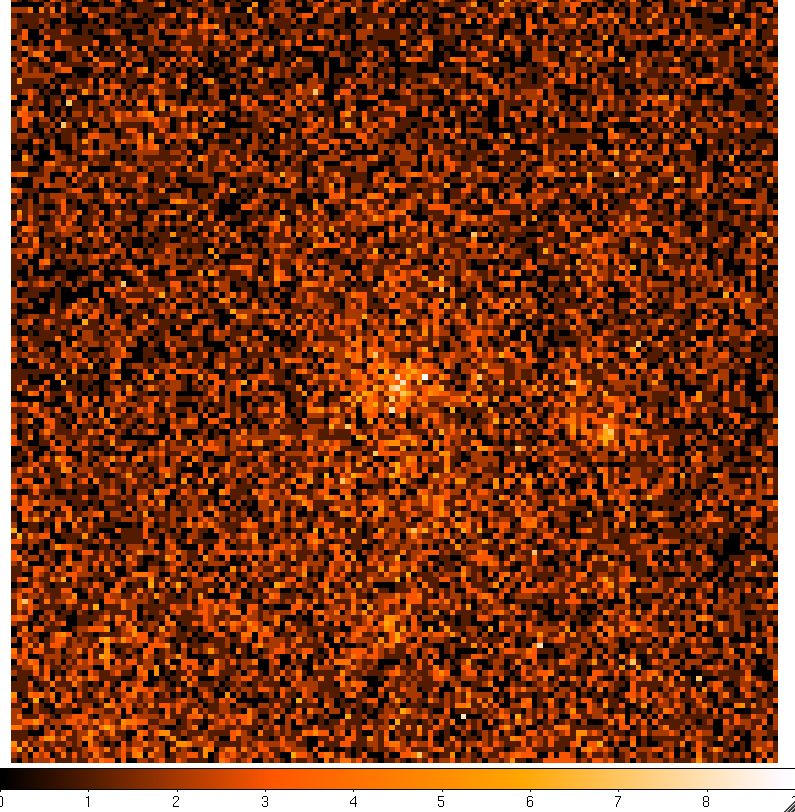
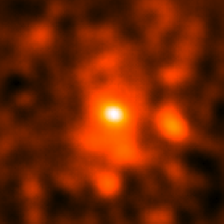
Visualizing the lobes with this raw image is not easy. You can kind of see some emission in the center but not really resolve it. However, if you can smooth this image in ds9 by clicking the 'Analysis Menu' and then selecting 'Smooth'. This is better, but not quite good enough. So click 'Analysis' again and select 'Smooth Parameters'. This should bring up a dialog box where you can select the Kernel Radius. Set this to 9 and click 'Apply' and then close the dialog box. The resulting image is pretty washed out now so click 'Color' and then select 'b'. If you play with the color scale by holding the right mouse button while dragging it around you can wind up with a smoothed count map that looks a little like the one in the publication:

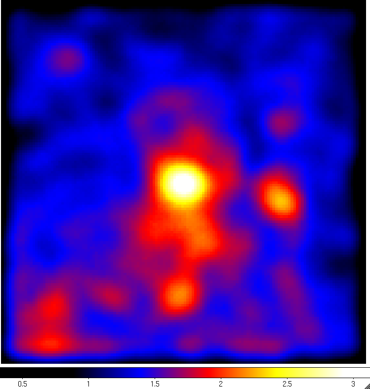
We're not going to get something perfect here since we're manually playing with the color scaling and the paper used a sophisticated adaptive smoothing algorithm while we're just using the simple gaussian algorithm included in ds9. However, you can already see the central core of CenA and some diffuse emission to the north and south of the core that kind of looks like extended emission. You can also see several point sources in the ROI that are other gamma-ray sources we'll need to model. Since Cen A is near the galactic plane you can make out some of the galactic diffuse emission at the bottom of the image.

Create a Template for the Extended Emission

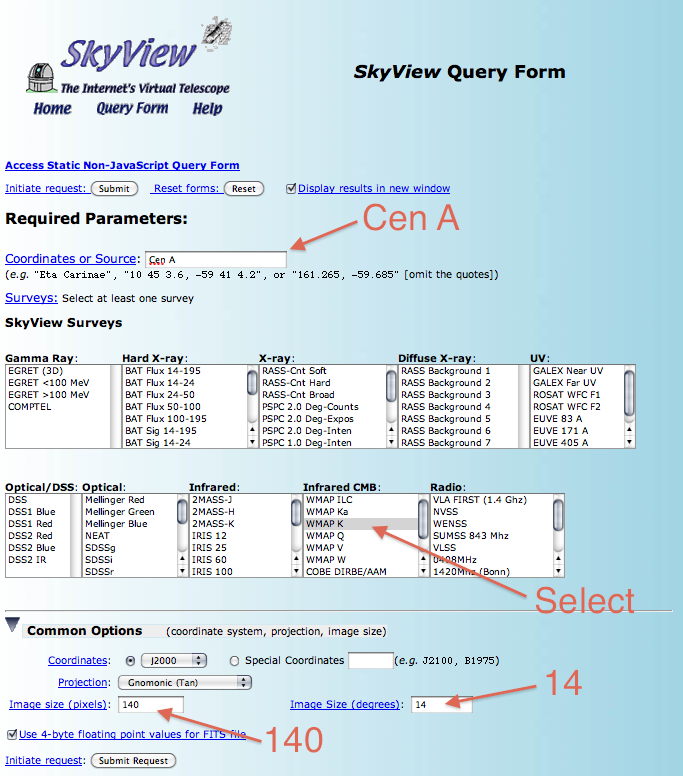
Now that we've convinced ourselves that there is extended lobe emission we need to find a way to describe the spatial extent. In this case we'll follow the example of the publication and use the WMAP k-band observations as a template. The exact WMAP template that was used in the publication is not available but we can get a very similar one from NASA's SkyView. Navigate to SkyView using and click on the SkyView Query Form link. We want to download the WMAP data in a region around Cen A so input 'Cen A' into the 'Coordinates of Source' box of the form. Then select 'WMAP K' in the 'Infrared CMB:' box. We need to match our ROI so under 'Common Options' input '140' as the 'Image size (pixels)' and 14 as the 'Image Size (degrees)'. Once you've input all of this, hit the 'Submit Request' button.

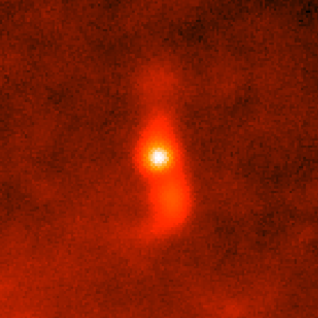
On the resulting page, you'll see an image of the WMAP data showing a fuzzy image of Cen A in the K-Band. This is nice but what we really want is the FITS image. So click the FITS link and download it into your working directory. In the following section we're going to assume that the SkyView image is called 'skv.fits' so rename the downloaded file accordingly. You can also download the WMAP image directly from us: skv.fits. Here's what the downloaded WMAP K-band image looks like in ds9 using the 'heat' color map and square-root scaling without any smoothing:

The raw image by itself is not in the correct form for the analysis we want to do. First of all, we want to subtract out the central core of Cen A and we want to divide the map into two parts so that we can seperately model the north and south lobes. Furthermore, there are a few things we need to do to make any map compatible with the Science Tools:

The template must be in J2000 coordinates. The likelihood code does not transpose coordinates into J2000.
The background must be set to 0. The likelihood code will use any pixel over 0 as part of the template.
The total flux must be normalized to 1.

The first point is already taken care of since the WMAP image is in J2000 coordinates. We'll take care of the second point by setting all of the points below a certain value to 0. This isn't the best way to do it but it's quick which is what we're going for in this thread. In the final step, we'll integrate over the entire map to get our normalization factor and divide each pixel by this number. So let's get started. We're going to use pyFits to do this which is included in the Science Tools (you could use a similar tools like IDL or ftools if you wanted). You can find more details on pyFits at the pyFits website.

Start up python, import the pyfits and math modules and open the WMAP image:


[user@localhost]$ python

Python 2.6.5 (r265:79063, Nov  9 2010, 12:49:33) 

[GCC 4.2.1 (Apple Inc. build 5664)] on darwin 

Type "help", "copyright", "credits" or "license" for more information.

>>> import pyfits

>>> import numpy as np

>>> wmap_image = pyfits.open('./skv.fits')

You can view the header of the image via the following command. The image is in the first HDU of the FITS file so you access the '0'th element of the wmap_image object.


>>> print wmap_image[0].header

...output suppressed...

Now we do a rough background suppression by setting any pixels less than 0.5 mK to 0. We'll also save the resulting image to a file so we can see what we've done.


>>> wmap_image[0].data[wmap_image[0].data < 0.5] = 0.0

>>> wmap_image.writeto('CenA_wmap_k_above5.fits')

If you open up this image in ds9 you'll notice that there's still some background left in the south east portion of the image so we'll get rid of this by setting any pixels that are more than 5 degrees away from the center to 0 and write this out to a file.

Remember that the image is 14 degrees and has a pixel size of 0.1 degrees. We're going to create a 2-d array that's filled with the distance to the center pixel.


>>> x = np.arange(-7,7,0.1)

>>> y = np.arange(-7,7,0.1)

>>> xx, yy = np.meshgrid(x, y, sparse=True)

>>> dist = np.sqrt(xx**2 + yy**2)

Now, set all of the pixels in the wmap data where dist is greater than 5 to 0.


>>> wmap_image[0].data[dist > 5] = 0.0

>>> wmap_image.writeto('CenA_wmap_k_nobkgrnd.fits')

The resulting image should only have emission from the radio galaxy left and the rest of the image set to 0. This is important because any non-zero pixels will be treated as part of the template by the likelihood code and will skew your results. Now we will continue on to subtract out the center 1 degree of the image so that the core of Cen A is not included in the template.


>>> wmap_image[0].data[dist < 1.0] = 0.0

>>> wmap_image.writeto('CenA_wmap_k_nocenter.fits')

At this point, we want to divide up our map into north and south pieces and normalize each of them. We need to normalize the flux of each template that we're using to 1. This means doing a two dimenstional integral over the image making sure to take into account the size of each bin. In practice, this means summing up all of the bins, multiplying this by (pi/180)^2 and multiplying this by the pixel area. We will now make the north map by setting all the south pixels to zero, normalize it and save it. We'll then close the image, open the image we saved before we did the zeroing out of the south pixels and do the same for the south region.


>>> wmap_image[0].data[0:69,0:140] = 0

>>> norm = np.sum(wmap_image[0].data) * (np.pi/180)**2 * (0.1**2)

>>> wmap_image[0].data = wmap_image[0].data / norm

>>> wmap_image.writeto('CenA_wmap_k_nocenter_N.fits')

>>> wmap_image.close()

Now open the file back up and do the same for the south region.


>>> wmap_image = pyfits.open("Cena_wmap_k_nocenter.fits")

>>> wmap_image[0].data[70:140,0:140]=0

>>> norm = np.sum(wmap_image[0].data) * (np.pi/180)**2 * (0.1**2)

>>> wmap_image[0].data = wmap_image[0].data / norm

>>> wmap_image.writeto('CenA_wmap_k_nocenter_S.fits')

>>> wmap_image.close()

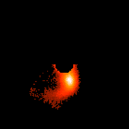
In the end, you should have two FITS files that look like the following images. The max value in the North template should be around 1670 and the max in the South should be around 900. If you are far away from these values, make sure you exectuted the above steps correctly.

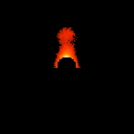Here are copies of the two templates:

CenA_wmap_k_nocenter_N.fits

CenA_wmap_k_nocenter_S.fits

Create a 3D Counts Map and Compute the Livetime

Now we can continue to follow the binned analysis prescription by creating a 3D counts map


[user@localhost]$ gtbin

This is gtbin version ScienceTools-v9r23p1-fssc-20110612
Type of output file (CCUBE|CMAP|LC|PHA1|PHA2) [] CCUBE

Event data file name[] CenA_filtered_gti.fits 

Output file name[] CenA_CCUBE.fits

Spacecraft data file name[] NONE

Size of the X axis in pixels[] 141

Size of the Y axis in pixels[] 141

Image scale (in degrees/pixel)[] 0.1

Coordinate system (CEL - celestial, GAL -galactic) (CEL|GAL) [] CEL

First coordinate of image center in degrees (RA or galactic l)[] 201.47

Second coordinate of image center in degrees (DEC or galactic b)[] -42.97

Rotation angle of image axis, in degrees[] 0

Projection method e.g. AIT|ARC|CAR|GLS|MER|NCP|SIN|STG|TAN:[] AIT

Algorithm for defining energy bins (FILE|LIN|LOG) [] LOG

Start value for first energy bin in MeV[] 210

Stop value for last energy bin in MeV[] 31000

Number of logarithmically uniform energy bins[] 20

Then compute the livetime. This will take something like 30 minutes to complete.


[user@localhost]$ gtltcube 

Event data file[] CenA_filtered_gti.fits 

Spacecraft data file[] SC.fits 

Output file[] CenA_ltcube.fits

Step size in cos(theta) (0.:1.) [] 0.025

Pixel size (degrees)[] 1

Working on file SC.fits

.....................!

Generate XML Model File

We have developed a model file (CenA_model.xml) based on the 2FGL that works for this ROI and the length of time of the observations. If you want to develop your own, you should look at the other threads where this is done. Also make sure you have the most recent galactic diffuse and isotropic model files which can be found at http://fermi.gsfc.nasa.gov/ssc/data/p7rep/access/lat/BackgroundModels.html.

Download the model file (CenA_model.xml) and put it in your working directory. If you open it up, you will see 13 background sources, the galactic and extragalactic backgrounds and the three sources of interest (CenA, CenA_NorthLobe and CenA_SouthLobe). Note that the Lobes reference the spatial models we created in the previous section (CenA_wmap_k_nocenter_N.fits and CenA_wmap_k_nocenter_S.fits).

For these three sources we are fitting a powerlaw model (see the Cicerone for descriptions of the different spectral and spatial models). The core of Cen A will be modeled by a point source (<spatialModel type="SkyDirFunction">) and the two lobes will be modeled using the templates we created from the WMAP sky map (<spatialModel file="some_map.fits" type="SpatialMap">).

Compute the Binned Exposure and Source Maps

Now, we need to compute a binned exposure map. Make sure you tell it 'none' when asked for a Counts cube so that you can choose the dimensions of the exposure map.


[user@localhost]$ gtexpcube2

Livetime cube file[] CenA_ltcube.fits
 
Counts map file[] none
 
Output file name[] CenA_BinnedExpMap.fits
 
Response functions to use[] P7REP_SOURCE_V15

Size of the X axis in pixels[] 400 

Size of the Y axis in pixels[] 400

Image scale (in degrees/pixel)[] 0.1

Coordinate system (CEL - celestial, GAL -galactic) (CEL|GAL) [] CEL
 
First coordinate of image center in degrees (RA or galactic l)[] 201.47

Second coordinate of image center in degrees (DEC or galactic b)[] -42.97

Rotation angle of image axis, in degrees[] 0 

Projection method e.g. AIT|ARC|CAR|GLS|MER|NCP|SIN|STG|TAN[] AIT

Start energy (MeV) of first bin[] 210

Stop energy (MeV) of last bin[] 31000

Number of logarithmically-spaced energy bins[] 20

Computing binned exposure map....................!

Note that we've matched the energy dimentsions of our binned exposure map to our counts cube but we've made it 40 degrees square instead of 14. This is so that gtsrcmaps can calculate the exposure on sources not in our ROI that still might contribute to emission within our ROI. To achieve this, gtsrcmaps finds the farthest point from the center of our ROI (i.e. one of the corners, a distance of 7*sqrt(2) degrees from the center) adds 10 degrees to this and then convolves the model counts map that it creates with the PSF. Since the PSF at low energies (100s of MeV) is on the order of 4 - 10 degrees in radius, we need to add an additional 10 degrees to account for the convolution. The total distance from the center in our case is thus 7*sqrt(2) + 10 + (4-10) or approximately 24 - 30 degrees. This means the smallest square region that can contain this circle is approximately 34 - 43 degrees on a side ((radius/sqrt(2))*2)). Don't worry about getting it exactly right, gtscrmaps will fail with an error about 'emapbnds' if you input an exposure cube that's too small and you can go back and make it larger.

Now we run gtsrcmaps to generate a source map using the model file we just created


[user@localhost]$ gtsrcmaps 

Exposure hypercube file[] CenA_ltcube.fits 

Counts map file[] CenA_CCUBE.fits 

Source model file[] CenA_model.xml 

Binned exposure map[] CenA_BinnedExpMap.fits

Source maps output file[] CenA_srcMaps.fits

Response functions[] CALDB

Generating SourceMap for CenA....................!

Generating SourceMap for CenA_NorthLobe....................!

Generating SourceMap for CenA_SouthLobe....................!

Generating SourceMap for _2FGLJ1259.8-3749....................!

Generating SourceMap for _2FGLJ1303.5-4622....................!

Generating SourceMap for _2FGLJ1304.3-4353....................!

Generating SourceMap for _2FGLJ1305.8-4925....................!

Generating SourceMap for _2FGLJ1306.9-4028....................!

Generating SourceMap for _2FGLJ1307.5-4300....................!

Generating SourceMap for _2FGLJ1311.7-3429....................!

Generating SourceMap for _2FGLJ1326.4-4729....................!

Generating SourceMap for _2FGLJ1328.5-4728....................!

Generating SourceMap for _2FGLJ1335.3-4058....................!

Generating SourceMap for _2FGLJ1347.7-3752....................!

Generating SourceMap for _2FGLJ1359.9-3746....................!

Generating SourceMap for _2FGLJ1417.5-4404....................!

Generating SourceMap for gal_2yearp7v6....................!

Generating SourceMap for iso_p7v6source....................!

Run the Likelihood Analysis

It's time to actually run the likelihood analysis now. First, you need to import the pyLikelihood module and then the BinnedAnalysis functions. As discussed in the likelihood thread it's best to do a two-pass fit here, the first with the MINUIT optimizer and a looser tolerance and then finally with the NewMinuit optimizer and a tighter tolerance. This allows us to zero in on the best fit parameters. For more details on the pyLikelihood module, check out the pyLikelihood Usage Notes.


>>> import pyLikelihood

>>> from BinnedAnalysis import *

>>> obs = BinnedObs(srcMaps='CenA_srcMaps.fits',expCube='CenA_ltcube.fits',binnedExpMap='CenA_BinnedExpMap.fits',irfs='CALDB')

>>> like1 = BinnedAnalysis(obs,'CenA_model.xml',optimizer='MINUIT')

Set the tolerance to something large to start out with, do the first fit and save the results to a file. Here, we get the minimization object (like1obj) from the logLike object so that we can access it later. We pass this object to the fit routine so that it knows which fitting object to use.


>>> like1.tol = 0.1

>>> like1obj = pyLike.Minuit(like1.logLike)

>>> like1.fit(verbosity=0,covar=True,optObject=like1obj)

86872.02278584728

>>> like1.logLike.writeXml('CenA_fit1.xml')

Let's check how the convergence of this first fit went.


>>> like1obj.getQuality()

2

This output corresponds to the MINUIT fit quality. A "good" fit corresponds to a value of "fit quality = 3"; if you get a lower value it is likely that there is a problem with the error matrix. According to the Minuit documentation possible values for "fit quality" are:

0 - Error matrix not calculated at all
1 - Diagonal approximation only, not accurate
2 - Full matrix, but forced positive-definite (i.e. not accurate)
3 - Full accurate covariance matrix (After MIGRAD, this is the indication of normal convergence.)

This is not that big of a deal right now since we are planning to fit this again with a tighter tolerance, but it's good to know that there might be problems with convergence. Now, create a new BinnedAnalysis object using the same BinnedObs object from before and the results of the previous fit and tell it to use the NewMinuit optimizer. We also double check that the tolerance is what we want (0.001) and then we fit the model and save the results.


>>> like2 =
BinnedAnalysis(obs,'CenA_fit1.xml',optimizer='NewMinuit')

>>> like2.tol = 1e-8

>>> like2obj = pyLike.NewMinuit(like2.logLike)

>>> like2.fit(verbosity=0,covar=True,optObject=like2obj)

86869.59660884333

>>> like2.logLike.writeXml('CenA_fit2.xml')

Now, check if NewMinuit converged.


>>> print like2obj.getRetCode()

0

The return codes for NewMinuit are different than those for Minuit (it's a bit mask). The only thing you really need to know is that if this number is anything but 0, the fit didn't converge. Now that we've done the full fit we can verify that we've gotten values close to what's in the publication. First check the results for the core:


>>> like2.Ts('CenA')

248.674472344

>>> like2.model['CenA']

CenA

   Spectrum: PowerLaw

0      Prefactor:  5.490e+00  6.228e-01  1.000e-04  1.000e+04 ( 1.000e-11)

1          Index:  2.684e+00  1.114e-01  0.000e+00  5.000e+00 (-1.000e+00)

2          Scale:  4.025e+02  0.000e+00  3.000e+01  5.000e+05 ( 1.000e+00) fixed

>>> like2.flux('CenA',emin=100,emax=100000)

1.36981632537e-07

>>> like2.fluxError('CenA',emin=100,emax=100000)

2.46676703398e-08

So, the core is detected with high significance (TS = 249) and the fit resulted in a spectral index of 2.7 +- 0.1. The integral flux above 100 MeV is (1.4 +- 0.2) x 10^-7. This matches well (within statistical errors) the index and flux reported in the article (index = 2.67 +- 0.10, flux = 1.50 +0.25/-0.22).

Now, check the north and south lobes.


>>> like2.Ts('CenA_NorthLobe')

76.25363991354243

>>> like2.model['CenA_NorthLobe']

CenA_NorthLobe

   Spectrum: PowerLaw

3      Prefactor:  3.552e+00  5.492e-01  1.000e-04  1.000e+04 ( 1.000e-11)

4          Index:  2.744e+00  2.284e-01  0.000e+00  5.000e+00 (-1.000e+00)

5          Scale:  4.362e+02  0.000e+00  3.000e+01  5.000e+05 ( 1.000e+00) fixed

>>> like2.flux('CenA_NorthLobe',emin=100,emax=100000)

1.1580928517071539e-07

>>> like2.fluxError('CenA_NorthLobe',emin=100,emax=100000)

3.3546535705124551e-08

>>> like2.Ts('CenA_SouthLobe')

254.8259087257611

>>> like2.model['CenA_SouthLobe']

CenA_SouthLobe

   Spectrum: PowerLaw

6      Prefactor:  7.177e+00  5.774e-01  1.000e-04  1.000e+04 ( 1.000e-11)

7          Index:  2.705e+00  1.088e-01  0.000e+00  5.000e+00 (-1.000e+00)

8          Scale:  4.362e+02  0.000e+00  3.000e+01  5.000e+05 ( 1.000e+00) fixed

>>> like2.flux('CenA_SouthLobe',emin=100,emax=100000)

2.257693623511771e-07

>>> like2.fluxError('CenA_SouthLobe',emin=100,emax=100000)

3.0256654573197757e-08

The north lobe is detected at a TS value of 76 while the south lobe is detected at a higher TS of 255. This is roughly what the LAT team reported. The north lobe has a spectral index of 2.7 +- 0.2 and an integral flux of (1.2 +- 0.3) x 10^-7. The south lobe has a spectral index of 2.7 +- 0.1 and an integral flux of (2.3 +- 0.3) x 10^-7. The integral fluxes are similar to what is reported in the paper (0.77 +0.23/-0.19 and 1.09 +0.24/-0.21 for the north and south lobes respectively) and still within statistical errors for the indices (2.52 +0.16/-0.19 for the north and 2.60 +0.14/-0.15 for the south). The main reasons for any discrepancy would be that we are using different IRFs, a slightly different template than was used by the LAT team and a different model file based on the 2FGL. The fact that our results are so close indicates that the method is robust. If you get results that are outside of the errors of the thread, double check that you've followed the thread accurately.

Create some Residual Maps

It's easiest to visualize our results by generating some model maps based on the model we just created and then use these models to create residuals maps based on the accual counts map. We're going to create four different model maps:

CenA_ModelMap_All.fits: A map of the full model (nothing commented out)
CenA_ModelMap_AllBkgrnd.fits: A map of all of the background sources (comment out the Cen A sources)
CenA_ModelMap_CenA.fits: A map of just the Cen A sources (comment out everything but the Cen A sources)
CenA_ModelMap_Diff.fits: A map of just the diffuse background sources (comment out everything but the isotropic and galactic sources)

To do this, we'll need to edit the output xml model file ('CenA_fit2.xml') each time and then run gtmodel. You don't need to edit it at all for the first one:


[user@localhost]$ gtmodel

Source maps (or counts map) file[] CenA_srcMaps.fits
 
Source model file[] CenA_fit2.xml 

Output file[] CenA_ModelMap_All.fits

Response functions[] CALDB

Exposure cube[] CenA_ltcube.fits 

Binned exposure map[] CenA_BinnedExpMap.fits

For the next file, comment out the Cen A sources in the xml file (you comment out text in xml using '' before and after the text you want to comment out) and run gtmodel again.


[user@localhost]$ gtmodel

Source maps (or counts map) file[] CenA_srcMaps.fits
 
Source model file[] CenA_fit2.xml 

Output file[] CenA_ModelMap_AllBkgrnd.fits

Response functions[] CALDB

Exposure cube[] CenA_ltcube.fits 

Binned exposure map[] CenA_BinnedExpMap.fits

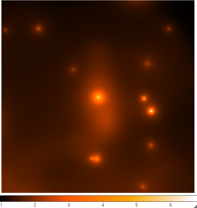
Continue to comment out select parts of the model xml file according to the list above and run gtmodel afterwards to get the next two files. You should end up with the four images below:


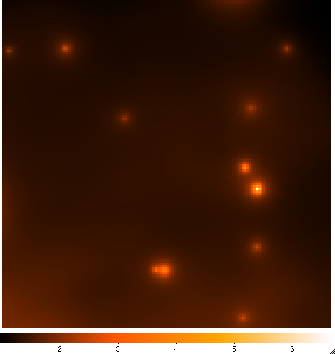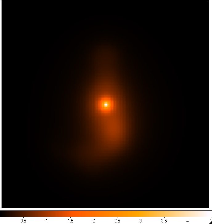
CenA_ModelMap_All.png: All of the sources in our model. You can see how the Cen A lobes are being modeled as well as numerous point sources and the diffuse backgrounds.	CenA_ModelMap_AllBkgrnd.png: Only the background sources. The CenA lobes and core are not in this image.

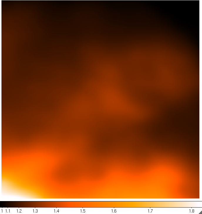CenA_ModelMap_CenA.png: Just the Cen A sources. This looks really nice.	CenA_ModelMap_Diffuse.png: Only the glactic and extragalactic diffuse emission. This is basically a blur in the background of all of our sky regions.

Now, we'll use the ftool, farith to subtract these model maps from our data to create residual maps.


[user@localhost]$ farith CenA_CMAP.fits CenA_ModelMap_All.fits CenA_CMAP_Resid.fits SUB

[user@localhost]$ farith CenA_CMAP.fits CenA_ModelMap_AllBkgrnd.fits CenA_CMAP_CenA.fits SUB

[user@localhost]$ farith CenA_CMAP.fits CenA_ModelMap_CenA.fits CenA_CMAP_Bkgrnd.fits SUB

[user@localhost]$ farith CenA_CMAP.fits CenA_ModelMap_Diff.fits CenA_CMAP_Sources.fits SUB

This should give you the following residual counts maps (smoothed with a 9 pixel gaussian like before):


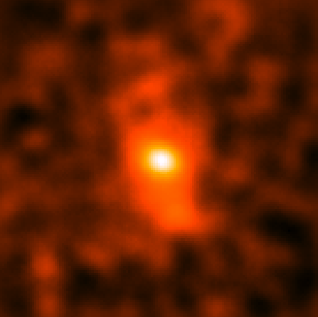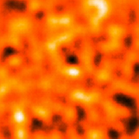
CenA_CMAP_Resid.png: Counts map minus all of the sources in the model showing that there's not really anything left after we subtract everything out.	CenA_CMAP_CenA.png: Everthing subtracted except the Cen A core and lobes. You can really see the extent of the radio galaxy in this map.

CenA_CMAP_Bkgrund.png: This shows a counts map with the Cen A core and lobes removed. The galaxtic and extragalactic emission dominates here but you can see a few individual point sources.	CenA_CMAP_Sources.png: This shows the region with the galactic and extragalactic emission removed so you can see the point sources along with the Cen A sources.

Finished

So, it looks like we've generally reproduced the results from the Cen A paper. You can go on from here and produce a proper spectrum using the model you have produced here (see the python likelihood thread) and you can plot a profile if you like (try using pyfits and matplotlib, both included in the science tools). You can also create any type of template you wish now to analyze extended diffuse sources using arbitrary shapes (create them in python and use pyfits to save them). Just make sure you follow the prescription outlined above.

Last updated by: Jeremy S. Perkins 05/07/2014

National Aeronautics and Space Administration

Goddard Space Flight Center