
Please Note: An updated, and maintained, version of this content is available on Github as a Jupyter notebook.
Fermi LAT Aperture Photometry
LAT light curves can be created in two different ways, either by using a likelihood analysis (see the Likelihood and Likelihood with Python tutorials) or through aperture photometry. A likelihood analysis is the more rigorous approach and offers the potential to reach greater sensitivity. It also leads to more accurate flux measurement, as backgrounds can be modeled out and more detailed source models can be applied. However, aperture photometry can also be useful – it provides a model independent measure of the flux, requires fewer analysis steps, and is less computationally demanding. It also enables the use of short time bins whereas likelihood analysis requires that time bins contain sufficient photons for analysis.
It is assumed that prior to working through this tutorial, you already have a familiarity with the concepts in the LAT Data Preparation and Data Exploration analysis threads. The basic steps for aperture photometry are described below. Although this is straightforward, there are several steps and so it may be convenient for them to be combined together into a script. An example of how this can be done is available in the User Contributions area. You will also need to have the FTOOLS software package installed.
In the example below a light curve is created centered on 3C 279. A 1-degree radius aperture is used with an energy range of 100 MeV to 200 GeV for the first 6 months of the Fermi mission. In this example the photon files obtained from the LAT Data Server are:
and the spacecraft file is:
Note: If you have downloaded your own files from the dataserver, your numbers may vary from those in this example.
You can download this tutorial as a Jupyter notebook and run it interactively. Please see the instructions for using the notebooks with the Fermitools.
Combine the Data Files
First, combine together the two photon files into a single file using gtselect. gtselect will be run again in a subsequent step with more selective constraints, but this shows its use for combining together multiple photon files. This approach can also be useful for combining together the weekly photon files which cover the entire sky. The file "events.txt" contains a list of the photon file names.
prompt> gtselect zmax=180 emin=100 emax=200000 infile=@events.txt outfile=tmp_19290temp1.fits ra=180 dec=0 rad=180 evclass=128 tmin=0 tmax=0
Next determine the start time of the photon file. Here we will use fkeypar, although other applications such as fv or gtvcut could be used as well.
prompt> fkeypar tmp_19290temp1.fits TSTART
Obtain this value with pget:
prompt>  pget fkeypar value

239557417.
Determine the stop time of the photon file using fkeypar:
prompt> fkeypar tmp_19290temp1.fits TSTOP
and obtain the value:
prompt> pget fkeypar value

255335917.
Select the desired event class
An output file filtered on LAT event class is then created which is used in subsequent steps. To do that you have to run the gtselect tool (see the example in the Data Preparation tutorial. With this tool you can also select events based on the aperture, energy range, and zenith distance, and output the results to a new file. The start and stop times determined above are needed for this step. We should trim these times by about a minute on either side, to allow us to barycenter the data later.
prompt> gtselect zmax=90 emin=100 emax=200000 infile=tmp_19290temp1.fits outfile=tmp_19290temp2.fits ra=194.046527 dec=-5.789312 rad=1 tmin=239557517 tmax=255335817 evclass=128
For aperture photometry we select a very small aperture (rad=1 degree), because we are not fitting the background. A tight ROI should exclude most background events and focuses on the events that are most likely to have originated from our source of interest. This data selection is significantly different from that used for likelihood analysis. Running gtselect generates a file with the correct events selected, but without exposure corrections for that event subset.
Set the good time intervals for these selections by using gtmktime on the temporary file you created with gtselect. This uses the offset angle from the aperture and the zenith, as well as the angle of the aperture from the center of the LAT field of view to exclude times when your source is too close to the Earth's limb. It also excludes times when the source is within 5 degrees of the Sun. This can be important for times when the Sun is active. gtmktime creates another output file:
prompt> gtmktime scfile=L1506171513514365357F56_SC00.fits filter="(DATA_QUAL==1) && ABS(ROCK_ANGLE)<90 && (LAT_CONFIG==1) && (angsep(RA_ZENITH,DEC_ZENITH,194.046527,-5.789312)+1<105) && (angsep(194.046527,-5.789312,RA_SUN,DEC_SUN)>5+1) &&(angsep(194.046527,-5.789312,RA_SCZ,DEC_SCZ)<180)" roicut=yes evfile=tmp_19290temp2.fits outfile=tmp_19290temp3.fits
The result is a new file (tmp_19290temp3.fits) with the correct events selected as well as the proper GTIs for those selections.
Create the Light Curve
Next you need to use gtbin to create the light curve with the desired time binning. In this case we have selected linear binning with a bin width (dtime) of 86400 seconds (=1 day).
prompt> gtbin algorithm=LC evfile=tmp_19290temp3.fits outfile=lc_3C279.fits scfile=L1506171513514365357F56_SC00.fits tbinalg=LIN tstart=239557517 tstop=255335817 dtime=86400
This produces a binned lightcurve file: lc_3C279.fits
Now you should determine the exposure for each time bin using gtexposure. This is the most computationally intensive and time consuming step, as the tool generates the exposure for each time bin and writes it to a new column in your file. In the example below, a source powerlaw index of 2.1 is used. If a more accurate spectral index is known for your source, then you should use that value instead.
prompt> gtexposure infile=lc_3C279.fits scfile=L1506171513514365357F56_SC00.fits irfs=P8R3_SOURCE_V2 srcmdl="none" specin=-2.1
If desired, the light curve can now be barycenter corrected using gtbary. This is only required if the time bins used are small and it is desired to investigate short timescale variability. It is important that gtbary is run after, and not before, the exposure correction is made.
prompt> gtbary evfile=lc_3C279.fits outfile=lc_3C279_bary.fits scfile=L1506171513514365357F56_SC00.fits ra=194.046527 dec=-5.789312 tcorrect=BARY
NOTE: If you did not trim a bit of time off either end of your data set, you will get the following error here:
Caught St13runtime_error at the top level: Cannot get Fermi spacecraft position for 239557417 Fermi MET (TT): the time is not covered by spacecraft file L1506171513514365357F56_SC00.fits[SC_DATA]This is because the spacecraft file uses 30-second gridding within your time range, and gtbary needs data points outside your time range to provide the reference information for the tool to use for the barycentering calculation.
You now have a light curve with counts per time bin. Note that the columns in the output file do not include a rate or a rate error column. So, in order to obtain photons/cm2/s it will be necessary to divide the COUNTS column by the EXPOSURE column. This can be accomplished, e.g. with the fv application or by using ftcalc as shown here.
prompt> ftcalc lc_3C279.fits lc_3C279_rate.fits RATE 'counts/exposure'


prompt> ftcalc lc_3C279_rate.fits lc_3C279_rate_error.fits RATE_ERROR 'error/exposure'
Here is an example light curve for 3C 279 obtained from aperture photometry for the first 6 months of the mission.
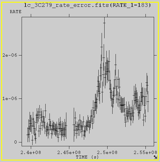
Note: The light curves obtained from aperture photometry procedure described above are NOT background subtracted. To obtain the background it will be necessary to model the sources in the region using a likelihood method. For some purposes (such as periodicity searches) background subtraction may not be necessary, and aperture photometry is appropriate.
Event Weighting
You may wish to use the gtsrcprob tool to assign probabilities to each event based on an input source model (such as the one used in the likelihood analysis. This can improve your lightcurve by increasing your acceptance radius whie selecting only events that are likely to have originated from your source.
To do this, first perform a likelihood analysis for your source for the time period that interests you. This process includes calculating the diffuse responses for each event, which has already been done for the data in the tmp_19290temp3.fits file.
The output XML file from the likelihood analysis is an input for gtsrcprob, but should be modified so that no source name contains a space, or begins with a number. Now run gtsrcprob to generate probabilities that each event may originate from each of the four modeled sources (src_3C_279, src_3C_273, Galactic Diffuse, and Isotropic Diffuse). You may need to download the latest diffuse models prior to running gtsrcprob. All of the most up-to-date background models along with a description of the models are available here
Note: Since gtsrcprob is a function of likelihood, it should not be used as a precursor to other likelihood analyses.
prompt> gtsrcprob evfile=tmp_19290temp3.fits scfile=L1506171513514365357F56_SC00.fits outfile=3C279_srcprob.fits srcmdl=3C279_output_model.xml irfs=P8R3_SOURCE_V2
Your output file, 3C279_srcprob.fits now contains four new columns with the probabilities for each event. You can now filter this file and retain only events with a high probability (in this case, > 80%) of being from 3C 279.
prompt> ftselect 3C279_srcprob.fits 3C279_srcprob_80.fits 'src_3C_279>0.8'
The resulting file can then be used as described above to create a light curve.
Last updated by: N. Mirabal 10/04/2018

- Curator: J.D. Myers
- NASA Official: Elizabeth Hays
- Fermi FAQ, Comments, Feedback
- › Privacy Policy and Important Notices
- › Accessibility
- › Contact NASA
- › Page Last Updated: Mon, Sep 08, 2025