National Aeronautics and Space Administration

Goddard Space Flight Center

Data

• Data Policy
• Data Access
• Data Analysis

• Caveats
• Newsletters
• FAQ

Likelihood Analysis with Python

The python likelihood tools are a very powerful set of analysis tools that expand upon the command line tools provided with the Fermitools package. Not only can you perform all of the same likelihood analysis with the python tools that you can with the standard command line tools but you can directly access all of the model parameters. You can more easily script a standard analysis like light curve generation. There are also a few things built into the python tools that are not available from the command line like the calculation of upper limits.

There are many user contributed packages built upon the python backbone of the Fermitools and we are going to highlight and use a few of them in this tutorial like likeSED, LATSourceModel, and the LATAnalysisScripts.

This sample analysis is based on the PG 1553+113 analysis performed by the LAT team and described in Abdo, A. A. et al. 2010, ApJ, 708, 1310. At certain points we will refer to this article as well as the Cicerone. After you complete this tutorial you should be able to reproduce all of the data analysis performed in this publication including generating a spectrum (individual bins and a butterfly plot) and produce a light curve with the python tools. This tutorial assumes you have the most recent Fermitools installed. We will also make significant use of python, so you might want to familiarize yourself with python (there's a beginner's guide at http://wiki.python.org/moin/BeginnersGuide). This tutorial also assumes that you've gone through the non-python based unbinned likelihood thread. This tutorial should take approximately 8 hours to complete (depending on your computer's speed) if you do everything but there are some steps you can skip along the way which shave off about 4 hours of that.

Note: In this tutorial, commands that start with '[user@localhost]$' are to be executed within a shell environment (bash, c-shell etc.) while commands that start with '>>>' are to be executed within an interactive python environment. Commands are in bold and outputs are in normal font. Text in ITALICS within the boxes are comments from the author.

You can download this tutorial as a Jupyter notebook and run it interactively. Please see the instructions for using the notebooks with the Fermitools.

Get the Data

For this thread the original data were extracted from the LAT data server with the following selections (these selections are similar to those in the paper):

• Search Center (RA,Dec) = (238.929,11.1901)
• Radius = 20 degrees
• Start Time (MET) = 239557417 seconds (2008-08-04T15:43:37)
• Stop Time (MET) = 256970880 seconds (2009-02-22T04:48:00)
• Minimum Energy = 100 MeV
• Maximum Energy = 300000 MeV

We've provided direct links to the event files as well as the spacecraft data file if you don't want to take the time to use the download server. For more information on how to download LAT data please see the Extract LAT Data tutorial.

• L1504241622054B65347F25_PH00.fits
• L1504241622054B65347F25_PH01.fits
• L1504241622054B65347F25_SC00.fits

You'll first need to make a file list with the names of your input event files:

[user@localhost]$ ls -1 *PH*.fits > PG1553_events.list

In the following analysis we've assumed that you've named your list of data files PG1553_events.list and the spacecraft file PG1553_SC.fits.

Perform Event Selections

You could follow the unbinned likelihood tutorial to perform your event selections using gtlike, gtmktime etc. directly from the command line, and then use pylikelihood later. But we're going to go ahead and use python. The gt_apps module provides methods to call these tools from within python. This'll get us used to using python.

So, let's jump into python:

[user@localhost]$ python
Python 2.7.8 (default, Apr 8 2015, 02:38:01)
[GCC 4.4.7 20120313 (Red Hat 4.4.7-4)] on linux2
Type "help", "copyright", "credits" or "license" for more information.
>>>

Ok, we want to run gtselect inside but we first need to import the gt_apps module to gain access to it.

>>> import gt_apps as my_apps

Now, you can see what objects are part of the gt_apps module by executing:

>>> help(my_apps)


Which brings up the help documentation for that module (type 'x' to exit). The python object for gtselect is called filter and we first need to set all of it's options. This is very similar to calling gtselect form the command line and inputting all of the variables interactively. It might not seem that convenient to do it this way but it's really nice once you start building up scripts and reading back options and such. For example, towards the end of this thread, we'll want to generate a light curve and we'll have to run the likelihood analysis for each datapoint. It'll be much easier to do all of this within python and change the tmin and tmax in an iterative fashion. Note that these python objects are just wrappers for the standalone tools so if you want any information on their options, see the corresponding documentation for the standalone tool.

>>> my_apps.filter['evclass'] = 128
>>> my_apps.filter['evtype'] = 3
>>> my_apps.filter['ra'] = 238.929
>>> my_apps.filter['dec'] = 11.1901
>>> my_apps.filter['rad'] = 10
>>> my_apps.filter['emin'] = 100
>>> my_apps.filter['emax'] = 300000
>>> my_apps.filter['zmax'] = 90
>>> my_apps.filter['tmin'] = 239557417
>>> my_apps.filter['tmax'] = 256970880
>>> my_apps.filter['infile'] = '@PG1553_events.list'
>>> my_apps.filter['outfile'] = 'PG1553_filtered.fits'


Once this is done, run gtselect:

>>> my_apps.filter.run()


Note that you can see exactly what gtselect will do if you run it by typing:

>>> my_apps.filter.command()


You have access to any of the inputs by directly accessing the filter['OPTIONS'] options.

Next, you need to run gtmktime. This is accessed within python via the maketime object:

>>> my_apps.maketime['scfile'] = 'PG1553_SC.fits'
>>> my_apps.maketime['filter'] = '(DATA_QUAL>0)&&(LAT_CONFIG==1)'
>>> my_apps.maketime['roicut'] = 'no'
>>> my_apps.maketime['evfile'] = 'PG1553_filtered.fits'
>>> my_apps.maketime['outfile'] = 'PG1553_filtered_gti.fits'
>>> my_apps.maketime.run()


We're using the most conservative and most commonly used cuts described in deatil in the Cicerone.

Livetime Cubes and Exposure Maps

At this point, you could make a counts map of the events we just selected using gtbin (it's called evtbin within python) and I won't discourage you but we're going to go ahead and create a livetime cube and exposure map. This might take a few minutes to complete so if you want to create a counts map and have a look at it, get these processes going and open another terminal to work on your counts map (see the likelihood tutorial for an example of running gtbin to produce a counts map).

Livetime Cube

This step will take approximately 15 - 30 minutes to complete so if you want to just download the PG1553_ltCube from us you can skip this step.

>>> my_apps.expCube['evfile'] = 'PG1553_filtered_gti.fits'
>>> my_apps.expCube['scfile'] = 'PG1553_SC.fits'
>>> my_apps.expCube['outfile'] = 'PG1553_ltCube.fits'
>>> my_apps.expCube['zmax'] = 90
>>> my_apps.expCube['dcostheta'] = 0.025
>>> my_apps.expCube['binsz'] = 1
>>> my_apps.expCube.run()



While you're waiting, you might have noticed that not all of the command line Fermitools have an equivalent object in gt_apps. This is easy to fix. Say you want to use gtltcubesun from within python. Just make it a GtApp:

>>> from GtApp import GtApp
>>> expCubeSun = GtApp('gtltcubesun','Likelihood')
>>> expCubeSun.command()


Exposure Map

>>> my_apps.expMap['evfile'] = 'PG1553_filtered_gti.fits'
>>> my_apps.expMap['scfile'] = 'PG1553_SC.fits'
>>> my_apps.expMap['expcube'] = 'PG1553_ltCube.fits'
>>> my_apps.expMap['outfile'] = 'PG1553_expMap.fits'
>>> my_apps.expMap['irfs'] = 'CALDB'
>>> my_apps.expMap['srcrad'] = 20
>>> my_apps.expMap['nlong'] = 120
>>> my_apps.expMap['nlat'] = 120
>>> my_apps.expMap['nenergies'] = 37
>>> my_apps.expMap.run()


Generate XML Model File

We need to create an XML file with all of the sources of interest within the Region of Interest (ROI) of PG 1553+113 so we can correctly model the background. For more information on the format of the model file and how to create one, see the likelihood analysis tutorial. For this thread, we use a simplified model with just two sources PG1553compact_model.xml. To fit all 4FGL-DR3 sources, you can use the user contributed LATSourceModel package to create a model file based on the LAT 14-year LAT catalog. You'll need to download the XML or FITS version of this file at http://fermi.gsfc.nasa.gov/ssc/data/access/lat/14yr_catalog/ and put it in your working directory. You will also need to install the LATSourceModel package (see also this page). Also make sure you have the most recent galactic diffuse and isotropic model files which can be found at http://fermi.gsfc.nasa.gov/ssc/data/access/lat/BackgroundModels.html. The catalog and background models are packaged with your installation of the Fermitools, which can be found at: $FERMI_DIR//refdata/fermi/galdiffuse/.

Once you have all of the files, you can generate your model file in python:

>>> from LATSourceModel import SourceList
>>> source_list = SourceList(catalog_file='gll_psc_v32.xml',ROI='PG1553_filtered_gti.fits',output_name='PG1553_model.xml',DR=4)
>>> source_list.make_model()
Creating spatial and spectral model from the 4FGL DR-4 catalog: gll_psc_v32.xml.
Added 164 point sources and 0 extended sources.
Building ds9-style region file...done!
File saved as ROI_PG1553_model.reg.


For more information on the LATSourceModel package, see the installation & usage notes.

In the paper, the LAT team only included two sources; one from the 0FGL catalog and another, non-catalog source. This is because the later LAT catalogs had not been released at the time. For a more updated model, one should use the latest 4FGL-DR4 information.

Back to looking at our compact XML model file, notice that PG 1553+113 is listed in the model file as 4FGL J1555.7+1111 with all of the parameters filled in for us. It's actually offset from the center of our ROI by 0.003 degrees. How nice! Also notice that we changed the model for 4FGL J1555.7+1111 from a Log Parabola to a simple power-law for the purposes of this analysis thread.

Compute the diffuse source responses.

The diffuse source responses tell the likelihood fitter what the expected contribution would be for each diffuse source, given the livetime associated with each event. The source model XML file must contain all of the diffuse sources to be fit. The gtdiffrsp tool will add one column to the event data file for each diffuse source. The diffuse response depends on the instrument response function (IRF), which must be in agreement with the selection of events, i.e. the event class and event type we are using in our analysis. Since we are using SOURCE class, CALDB should use the P8R3_SOURCE_V3 IRF for this tool.

If the diffuse responses are not precomputed using gtdiffrsp, then the gtlike tool will compute them at runtime (during the next step). However, as this step is very computationally intensive (often taking ~hours to complete), and it is very likely you will need to run gtlike more than once, it is probably wise to precompute these quantities.

>>> my_apps.diffResps['evfile'] = 'PG1553_filtered_gti.fits'
>>> my_apps.diffResps['scfile'] = 'PG1553_SC.fits'
>>> my_apps.diffResps['srcmdl'] = 'PG1553compact_model.xml'
>>> my_apps.diffResps['irfs'] = 'CALDB'
>>> my_apps.diffResps.run()


Run the Likelihood Analysis

It's time to actually run the likelihood analysis now. First, you need to import the pyLikelihood module and then the UnbinnedAnalysis functions (there's also a binned analysis module that you can import to do binned likelihood analysis which behaves almost exactly the same as the unbinned analysis module). For more details on the pyLikelihood module, check out the pyLikelihood Usage Notes.

>>> import pyLikelihood
>>> from UnbinnedAnalysis import *
>>> obs = UnbinnedObs('PG1553_filtered_gti.fits','PG1553_SC.fits',expMap='PG1553_expMap.fits',
expCube='PG1553_ltCube.fits',irfs='CALDB')
>>> like = UnbinnedAnalysis(obs,'PG1553compact_model.xml',optimizer='NewMinuit')


By now, you'll have two objects, 'obs', an UnbinnedObs object and like, an UnbinnedAnalysis object. You can view these objects attributes and set them from the command line in various ways. For example:

>>> print(obs)
Event file(s): PG1553_filtered_gti.fits
Spacecraft file(s): PG1553_SC.fits
Exposure map: PG1553_expMap.fits
Exposure cube: PG1553_ltCube.fits
IRFs: CALDB
>>> print(like)
Event file(s): PG1553_filtered_gti.fits
Spacecraft file(s): PG1553_SC.fits
Exposure map: PG1553_expMap.fits
Exposure cube: PG1553_ltCube.fits
IRFs: CALDB
Source model file: PG1553compact_model.xml
Optimizer: NewMinuit

or you can get directly at the objects attributes and methods by:

>>> dir(like)
['NpredValue', 'Ts', 'Ts_old', '__call__', '__class__', '__delattr__', '__dict__', '__doc__', '__format__', '__getattribute__', '__getitem__', '__hash__', '__init__', '__module__', '__new__', '__reduce__', '__reduce_ex__', '__repr__', '__setattr__', '__setitem__', '__sizeof__', '__str__', '__subclasshook__', '__weakref__', '_errors', '_importPlotter', '_inputs', '_isDiffuseOrNearby', '_minosIndexError', '_npredValues', '_plotData', '_plotResiduals', '_plotSource', '_renorm', '_separation', '_setSourceAttributes', '_srcCnts', '_srcDialog', '_xrange', 'addSource', 'covar_is_current', 'covariance', 'deleteSource', 'disp', 'e_vals', 'energies', 'energyFlux', 'energyFluxError', 'fit', 'flux', 'fluxError', 'freePars', 'freeze', 'getExtraSourceAttributes', 'logLike', 'maxdist', 'minosError', 'model', 'nobs', 'normPar', 'observation', 'oplot', 'optObject', 'optimize', 'optimizer', 'par_index', 'params', 'plot', 'plotSource', 'plotSourceFit', 'reset_ebounds', 'resids', 'restoreBestFit', 'saveCurrentFit', 'scan', 'setFitTolType', 'setFreeFlag', 'setPlotter', 'setSpectrum', 'sourceFitPlots', 'sourceFitResids', 'sourceNames', 'srcModel', 'state', 'syncSrcParams', 'thaw', 'tol', 'tolType', 'total_nobs', 'writeCountsSpectra', 'writeXml']

or get even more details by executing:

>>> help(like)


There are a lot of attributes and here you start to see the power of using pyLikelihood since you'll be able (once the fit is done) to access any of these attributes directly within python and use them in your own scripts. For example, you can see that the like object has a 'tol' attribute which we can read back to see what it is and then set it to what we want it to be.

>>> like.tol
0.001
>>> like.tolType
The tolType can be '0' for relative or '1' for absolute.
1
>>> like.tol = 0.0001
Now, we're ready to do the actual fit. This next step can take anywhere from 10 minutes to a few hours to complete, depending on your system. We're doing something a bit fancy here. We're getting the minimizating object (and calling it 'likeobj') from the logLike object so that we can access it later. We pass this object to the fit routine so that it knows which fitting object to use. We're also telling the code to calculate the covariance matrix so we can get at the errors.

>>> likeobj = pyLike.NewMinuit(like.logLike)
>>> like.fit(verbosity=0,covar=True,optObject=likeobj)
569867.6200552832

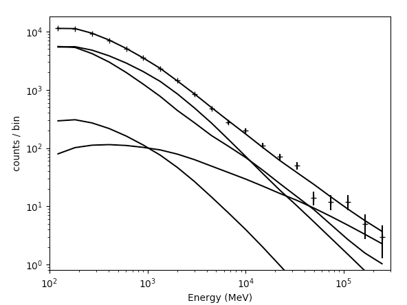
The number that is printed out here is the -log(Likelihood) of the total fit to the data. You can print the results of the fit by accessing like.model. You can now plot the results of the fit by executing the plot command. The results are shown below:

>>> like.plot()

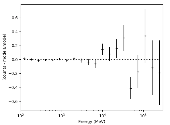The output of the plot function of the like1 UnbinnedAnalysis object shows:

• Left: the contribution of each of the objects in the model to the total model, and plots the data points on top.
• Right: the residuals of the likelihood fit to the data.Notice that the fit is poor in the second to last bin.

Now, check if NewMinuit converged.

>>> likeobj.getRetCode()
0

If you get anything other than '0' here, than NewMinuit didn't converge. There are several reasons that we might not get convergance:

• The culprit is usually a parameter (or parameters) in the model that reach the limits set in the XML file. If this happens the minimizer cannot reach the formal minimum, and hence cannot calculate the curvature.
• Often the problem is with spectral shape parameters (PL index etc..), so simply freezing the shape of all spectral parameters to their values from the full time period (and certainly for weaker background sources) when fitting a shorter time period may solve the problem. Remember that the 4FGL-DR3 catalog used a full 12 years of data and we're using a much shorter time period here
• Weak background sources are more likely to cause problems, so you could consider just freezing them completely (or removing them from the model). For example a background source from the catalog that is detected at TS~=25 in 2 years could cause convergence problems in a 1-month light curve, where it will often not be detectable at all.
• If there are no parameters at their limits, then increasing the overall convergence tolerance may help - try using a value of 1E-8 for the absolute tolerance.
• If that doesn't help then try to systematically simplify the model. Progressively freeze all sources, starting with those at the edge of the ROI in and moving in until you get a model simple enough for the minimizer to work reliably. For example if you are using a 10 degree ROI, you could start by freezing all background sources further than 7 degrees from the source of interest, and move to 5 degrees if that doesn't solve the problem.

In our case, we have convergence and can move forward. Note, however, that this doesn't mean you have the 'right' answer. It just means that you have the answer assuming the model you put in. This is a subtle feature of the likelihood method.

Let's take a look at the residuals and overal model using matplotlib.

>>> import matplotlib.pyplot as plt
>>> import numpy as np
We need to import these two modules for plotting and some other stuff. They are included in the Fermitools. >>> E = (like.energies[:-1] + like.energies[1:])/2.
The 'energies' array are the endpoints so we take the midpoint of the bins.
>>> plt.figure(figsize=(5,5))
>>> plt.ylim((0.4,1e4))
>>> plt.xlim((200,300000))
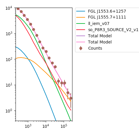
>>> sum_model = np.zeros_like(like._srcCnts(like.sourceNames()[0]))
>>> for sourceName in like.sourceNames():
>>>    sum_model = sum_model + like._srcCnts(sourceName)
>>>    plt.loglog(E,like._srcCnts(sourceName),label=sourceName[1:])
>>> plt.loglog(E,sum_model,label='Total Model')
>>> plt.errorbar(E,like.nobs,yerr=np.sqrt(like.nobs), fmt='o',label='Counts')
>>> ax = plt.gca()
>>> box = ax.get_position()
>>> ax.set_position([box.x0, box.y0, box.width * 0.5, box.height])
>>> plt.legend(bbox_to_anchor=(1.05, 1), loc=2, borderaxespad=0.)
>>> plt.show()
>>> resid = (like.nobs - sum_model)/sum_model
>>> resid_err = (np.sqrt(like.nobs)/sum_model)
>>> plt.figure(figsize=(9,9))
>>> plt.xscale('log')
>>> plt.errorbar(E,resid,yerr=resid_err,fmt='o')
>>> plt.axhline(0.0,ls=':')
>>> plt.show()


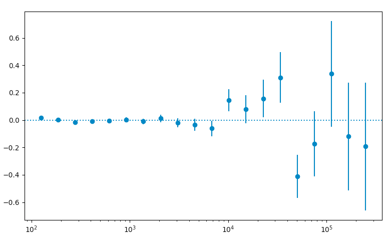
These are just some examples of how to access the underlying data from the python tools. As you can see, most of the information is accessable if you dig around. Note that the residuals aren't that great in several bins, especially at high energies. This could be a missing source or that we're not modelling a bright source very well. If you look up at the model plot, the high energy tail of PG1553 might be biasing the fit at high energies and we might get a better fit with a log-parabola or broken power-law. That's for another day though.

Let's check out the final parameters of the fit for PG1553.

>>> like.model['4FGL J1555.7+1111']
4FGL J1555.7+1111
Spectrum: PowerLaw
4 Prefactor: 3.052e+00 1.993e-01 1.000e-04 1.000e+04 ( 1.000e-11)
5 Index: 1.608e+00 2.884e-02 0.000e+00 1.000e+01 (-1.000e+00)
6 Scale: 5.000e+02 0.000e+00 3.000e+01 5.000e+05 ( 1.000e+00) fixed
>>> like.flux('4FGL J1555.7+1111',emin=100)
6.626736510332413e-08
>>> like.fluxError('4FGL J1555.7+1111',emin=100)
4.363836873328966e-09


You can also get the TS value for a specific source:

>>> like.Ts('4FGL J1555.7+1111')
2843.6311736518983


you can calculate how many standard deviations (σ) this corresponds to. (Remember that the TS value is ∼ σ².)

>>> np.sqrt(like.Ts('4FGL J1555.7+1111'))
53.325708374590754


Let's save the results.

>>> like.logLike.writeXml('PG1553_fit.xml')

Create some TS Maps

If you want to check on your fit you should probably make a test statistic (TS) map of your region at this point. This will allow you to check and make sure that you didn't miss anything in the ROI (like a source not in the catalog you used). A TS map is created by moving a putative point source through a grid of locations on the sky and maximizing the log(likelihood) at each grid point. We're going to make two TS Maps. If you have access to multiple CPUs, you might want to start one of the maps running in one terminal and the other in another one since this will take several hours to complete. Our main goal is to create one TS Map with PG1553 included in the fit and another without. The first one will allow us to make sure we didn't miss any sources in our ROI and the other will allow us to see the source. All of the other sources in our model file will be included in the fit and shouldn't show up in the final map.

If you don't want to create these maps, go ahead and skip the following steps and jump to the section on making a butterfly plot. The creation of these maps is optional and is only for double checking your work. You should still modify your model fit file as detailed in the following paragraph.

First open a new terminal and then copy PG1553_fit.xml as PG1553_fit_TSMap.xml. Modify PG1553_fit_TSMap.xml to make everything fixed by changing all of the free="1" statements to free="0". Modify the lines that look like:

to look like:

Then copy it and call it PG1553_fit_noPG1553.xml and comment out (or delete) the PG1553 source. If you want to generate the TS maps, in one window do the following:

>>> my_apps.TsMap['statistic'] = "UNBINNED"
>>> my_apps.TsMap['scfile'] = "PG1553_SC.fits"
>>> my_apps.TsMap['evfile'] = "PG1553_filtered_gti.fits"
>>> my_apps.TsMap['expmap'] = "PG1553_expMap.fits"
>>> my_apps.TsMap['expcube'] = "PG1553_ltCube.fits"
>>> my_apps.TsMap['srcmdl'] = "PG1553_fit_TSMap.xml"
>>> my_apps.TsMap['irfs'] = "CALDB"
>>> my_apps.TsMap['optimizer'] = "NEWMINUIT"
>>> my_apps.TsMap['outfile'] = "PG1553_TSmap_resid.fits"
>>> my_apps.TsMap['nxpix'] = 25
>>> my_apps.TsMap['nypix'] = 25
>>> my_apps.TsMap['binsz'] = 0.5
>>> my_apps.TsMap['coordsys'] = "CEL"
>>> my_apps.TsMap['xref'] = 238.929
>>> my_apps.TsMap['yref'] = 11.1901
>>> my_apps.TsMap['proj'] = 'STG'
>>> my_apps.TsMap.run()


In another window do the following:

>>> my_apps.TsMap['statistic'] = "UNBINNED"
>>> my_apps.TsMap['scfile'] = "PG1553_SC.fits"
>>> my_apps.TsMap['evfile'] = "PG1553_filtered_gti.fits"
>>> my_apps.TsMap['expmap'] = "PG1553_expMap.fits"
>>> my_apps.TsMap['expcube'] = "PG1553_ltCube.fits"
>>> my_apps.TsMap['srcmdl'] = "PG1553_fit_noPG1553.xml"
>>> my_apps.TsMap['irfs'] = "CALDB"
>>> my_apps.TsMap['optimizer'] = "NEWMINUIT"
>>> my_apps.TsMap['outfile'] = "PG1553_TSmap_noPG1553.fits"
>>> my_apps.TsMap['nxpix'] = 25
>>> my_apps.TsMap['nypix'] = 25
>>> my_apps.TsMap['binsz'] = 0.5
>>> my_apps.TsMap['coordsys'] = "CEL"
>>> my_apps.TsMap['xref'] = 238.929
>>> my_apps.TsMap['yref'] = 11.1901
>>> my_apps.TsMap['proj'] = 'STG'
>>> my_apps.TsMap.run()


This will take a while so go get a cup of coffee. The final TS maps will be pretty rough since we selected to only do 25x25 0.5 degree bins but it will allow us to check if anything is missing and go back and fix it. These rough plots aren't publication ready but they'll do in a pinch to verify that we've got the model right.

Once the TS maps have been generated, open them up in whatever viewing program you wish. Here's how you could use Matplotlib to do it.

>>> import astropy.io.fits as pyfits
>>> residHDU = pyfits.open('PG1553_TSmap_resid.fits')
>>> sourceHDU = pyfits.open('PG1553_TSmap_noPG1553.fits')
>>> fig = plt.figure(figsize=(16,8))
>>> plt.subplot(1,2,1)
>>> plt.imshow(residHDU[0].data)
>>> plt.colorbar()
>>> plt.subplot(1,2,2)
>>> plt.imshow(sourceHDU[0].data)
>>> plt.colorbar()
>>> plt.show()


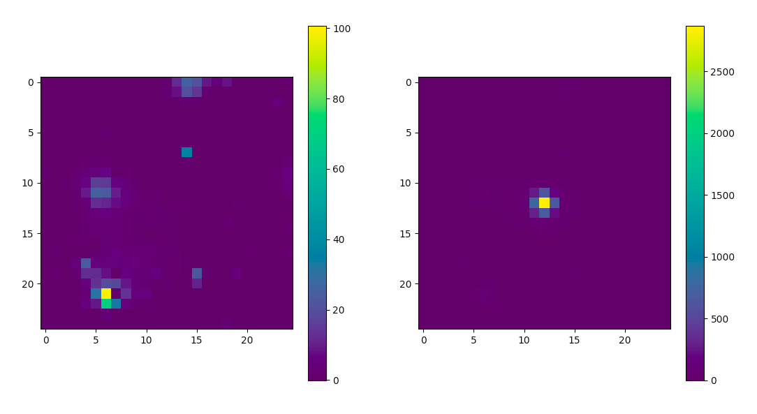
You can see that the 'noPG1553' map (right) has a prominent source in the middle of the ROI. This is PG 1553+113 and if you execute the following you can see that the TS value of the maxiumum pretty well with the TS value of PG 1553+113 that we arrived at above.

>>> np.max(sourceHDU[0].data)
2868.8123

If you then look at the 'residuals' plot (left), you can see that it's pretty flat in TS space. This indicates that we didn't miss any significant sources. If you did see something significant, you probably should go back and figure out what source you missed.

Produce the Butterfly Plot

Now we'll produce the butterfly plot. First, get the differential flux, the decorrelation (pivot) energy, and the index. You'll also need the errors.

>>> N0 = like.model['4FGL J1555.7+1111'].funcs['Spectrum'].getParam('Prefactor').value()
>>> N0_err = like.model['4FGL J1555.7+1111'].funcs['Spectrum'].getParam('Prefactor').error()
>>> gamma = like.model['4FGL J1555.7+1111'].funcs['Spectrum'].getParam('Index').value()
>>> gamma_err = like.model['4FGL J1555.7+1111'].funcs['Spectrum'].getParam('Index').error()
>>> E0 = like.model['4FGL J1555.7+1111'].funcs['Spectrum'].getParam('Scale').value()


Calculate the Butterfly Plot

We need to calculate the differential flux at several energy points as well as the error on that differential flux. The differential flux is defined as:

and the error on that flux is defined as:

Where cov_γγ = σ_γ², where γ is the spectral index. To calculate cov_γγ, use this code:

>>> freeParValues = []
>>> for sourcename in like.sourceNames():
>>>    for element in like.freePars(sourcename):
>>>       freeParValues.append(element.getValue())
>>>
>>> g_index = freeParValues.index(like.freePars('4FGL J1555.7+1111')[1].getValue())
>>> cov_gg = like.covariance[g_index][g_index]


So, let calculate F(E) and F(E) +/- Δ F(E) so that we can plot it. First, define a function for the flux and one for the error on the flux.

>>> f = lambda E,N0,E0,gamma: N0*(E/E0)**(-1*gamma)
>>> ferr = lambda E,F,N0,N0err,E0,cov_gg: F*np.sqrt(N0err**2/N0**2 + ((np.log(E/E0))**2)*cov_gg)


Now, generate some energies to evaluate the functions above and evaluate them.

>>> E = np.logspace(2,5,100)
>>> F = f(E,N0,E0,gamma)
>>> Ferr = ferr(E,F,N0,N0_err,E0,cov_gg)


Now you can plot this. Here we're multiplying the flux by E² for clarity.

>>> plt.figure(figsize=(8,8))
>>> plt.xlabel('Energy [MeV]')
>>> plt.ylabel(r'E$^2$ dN/dE [MeV s$^{-1}$ cm$^{-2}$]')
>>> plt.loglog(E,E**2*(F+Ferr))
>>> plt.loglog(E,E**2*(F-Ferr))
>>> plt.plot(E,E**2*F)
>>> plt.show()


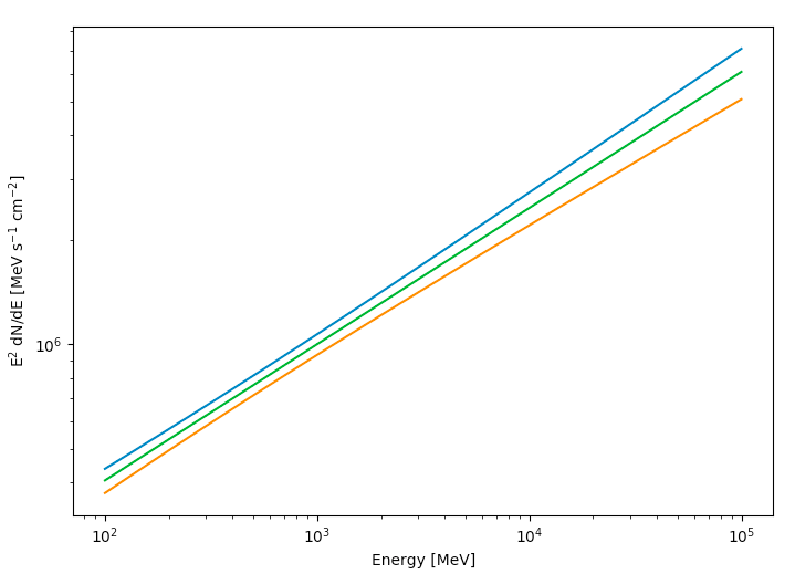
The green line is the nominal fit and the blue and orange lines are the 1 sigma contours.

---

Last updated by: J. Eggen 09/13/2023