
Unbinned Likelihood Tutorial
The detection, flux determination, and spectral modeling of Fermi LAT sources is accomplished by a maximum likelihood optimization technique as described in the Cicerone (see also e.g. Abdo, A. A. et al. 2009, ApJS, 183, 46). To illustrate how to use the Likelihood software, this narrative gives a step-by-step description for performing an unbinned likelihood analysis.
You can download this tutorial as a Jupyter notebook and run it interactively. Please see the instructions for using the notebooks with the Fermitools.
Unbinned vs Binned Likelihood
Unbinned likelihood analysis is the preferred method for time series analysis of the LAT data, where the number of events in each time bin is expected to be small.
However, for large time bins, analysis which includes bright background sources (such as the Galactic plane), and long time-baseline spectral and spatial analyses, a binned analysis is recommended.
To perform a binned likelihood analysis, see the Binned Likelihood tutorial.
Additional references:
- SciTools References
- Descriptions of available Spectral and Spatial Models
- Examples of XML Model Definitions for Likelihood:
Prerequisites
You will need an event data file, a spacecraft data file (also referred to as the "pointing and livetime history" file), and the current background models (available for download).
You may choose to select your own data files, or to use the files provided within this tutorial.
Custom data sets may be retrieved from the LAT Data Server.
Steps
Make Subselections from the Event Data
Since there is computational overhead for each event associated with each diffuse component, it is useful to filter out any events that are not within the extraction region used for the analysis.
Make Counts Maps from the Event Files
By making simple FITS images, we can inspect our data and pick out obvious sources.
Download the latest diffuse models
The recommended models for a normal point source analysis are
gll_iem_v07.fits(a very large file) andiso_P8R3_SOURCE_V3_v1.txt. All of the background models along with a description of the models are available here.
Create a Source Model XML File
The source model XML file contains the various sources and their model parameters to be fit using the gtlike tool.
Compute the diffuse responses
Each event must have a separate response precomputed for each diffuse component in the source model.
Make an Exposure Map
This is needed in order to analyze diffuse sources and derive absolute fluxes.
Perform the Likelihood Fit
Fitting the data to the model provides flux, errors, spectral indices, and other information.
Make Test-Statistic Maps
These are used for point source localization and for finding weaker sources after the stronger sources have been modeled.
1. Make Subselections from the event data
For this case the original extraction of data from the first six months of the mission was done as described in the Extract LAT Data tutorial.
Selection of data:
Search Center (RA, DEC) =(193.98, -5.82)
Radius = 20 degrees
Start Time (MET) = 239557417 seconds (2008-08-04 T15:43:37)
Stop Time (MET) = 255398400 seconds (2009-02-04 T00:00:00)
Minimum Energy = 100 MeV
Maximum Energy = 500000 MeV
We provide the user with the original photon and spacecraft data files extracted from the LAT Data Server:
L181204121625F588C43960_PH00.fits
L181204121625F588C43960_PH01.fits
L181204121625F588C43960_SC00.fits!wget https://fermi.gsfc.nasa.gov/ssc/data/analysis/scitools/data/dataPreparation/L181204121625F588C43960_PH00.fits
!wget https://fermi.gsfc.nasa.gov/ssc/data/analysis/scitools/data/dataPreparation/L181204121625F588C43960_PH01.fits
!wget https://fermi.gsfc.nasa.gov/ssc/data/analysis/scitools/data/dataPreparation/L181204121625F588C43960_SC00.fits
If you need to combine multiple events files for your analysis, you must first generate a text file listing the events files to be included.
!mkdir data
!mv *_PH* *_SC00* ./data
!mv ./data/*_SC00* ./data/spacecraft.fits
!ls ./data/*_PH* > ./data/events.txt
!cat ./data/events.txt
This text file (events.txt) will be used in place of the input fits filename when running gtselect. The syntax requires that you use an @ before the filename to indicate that this is a text file input rather than a fits file.
For simplicity, we rename the spacecraft file (the file ending in SC00) to spacecraft.fits.
When analyzing a point source, it is recommended that you include events with high probability of being photons. To do this, you should use gtselect to cut on the event class, keeping only the SOURCE class events (event class 128) (or as recommended in the Cicerone).
In addition, the full set of events have been divided into event types, which allow us to select events based on the conversion type, the quality of the track reconstruction, or the quality of the energy measurement. For standard selections, including all the event types for a given class, use evtype=3 ("INDEF" is the default in gtselect).
gtselect evclass=128 evtype=3
Be aware that evclass and evtype are hidden parameters. So to use them, you must type them on the command line.
We perform a selection to filter the data we want to analyze. For this example, we consider all SOURCE class events (i.e. evclass=128 and evtype=INDEF) within a 20 degree region of interest (ROI) centered on the blazar 3C 279. We apply the gtselect tool to the data file as follows:
%%bash
gtselect evclass=128 evtype=3
    @./data/events.txt
    ./data/3C279_region_filtered.fits
    193.98
    -5.82
    20
    INDEF
    INDEF
    100
    500000
    90
In the last step we also selected the energy range and the maximum zenith angle value (90 degrees). The Earth's limb is a strong source of background gamma rays. We filter them out with a zenith-angle cut. The value of 90 degrees is the one recommended by the LAT instrument team for analysis above 100 MeV. The filtered data are provided here.
After the data selection is made, we need to select the good time intervals in which the satellite was working in standard data taking mode and the data quality was good. For this task we use gtmktime to select GTIs by filtering on information provided in the spacecraft file. The current gtmktime filter expression recommended by the LAT team in the Cicerone is:
(DATA_QUAL>0)&&(LAT_CONFIG==1)This excludes time periods when some spacecraft event has affected the quality of the data, ensures the LAT instrument was in normal science data-taking mode.
Here is an example of running gtmktime for our analysis of the region surrounding 3C 279.
%%bash
gtmktime
    ./data/spacecraft.fits
    (DATA_QUAL>0)&&(LAT_CONFIG==1)
    no
    ./data/3C279_region_filtered.fits
    ./data/3C279_region_filtered_gti.fits
The data with all the cuts described above is provided in this link. A more detailed discussion of data selection can be found in the Data Preparation analysis thread.
To view the DSS keywords in a given extension of a data file, use the gtvcut tool and review the data cuts on the EVENTS extension. This provides a listing of the keywords reflecting each cut applied to the data file and their values, including the entire list of GTIs. Here we use the option suppress_gtis=yes to keep the output easily readable:
%%bash
gtvcut suppress_gtis=yes
    ./data/3C279_region_filtered_gti.fits
    EVENTS
Here you can see the event class selection, the location and radius of the data selection, the event type selection, as well as the energy range in MeV and the zenith angle cut. The time cuts to be used in the exposure calculation are defined by the GTI table.
Various Fermitools will be unable to run if you have multiple copies of a particular DSS keyword. This can happen if the position used in extracting the data from the data server is different than the position used with gtselect. It is wise to review the keywords for duplicates before proceeding. If you do have keyword duplication, it is advisable to regenerate the data file with consistent cuts.
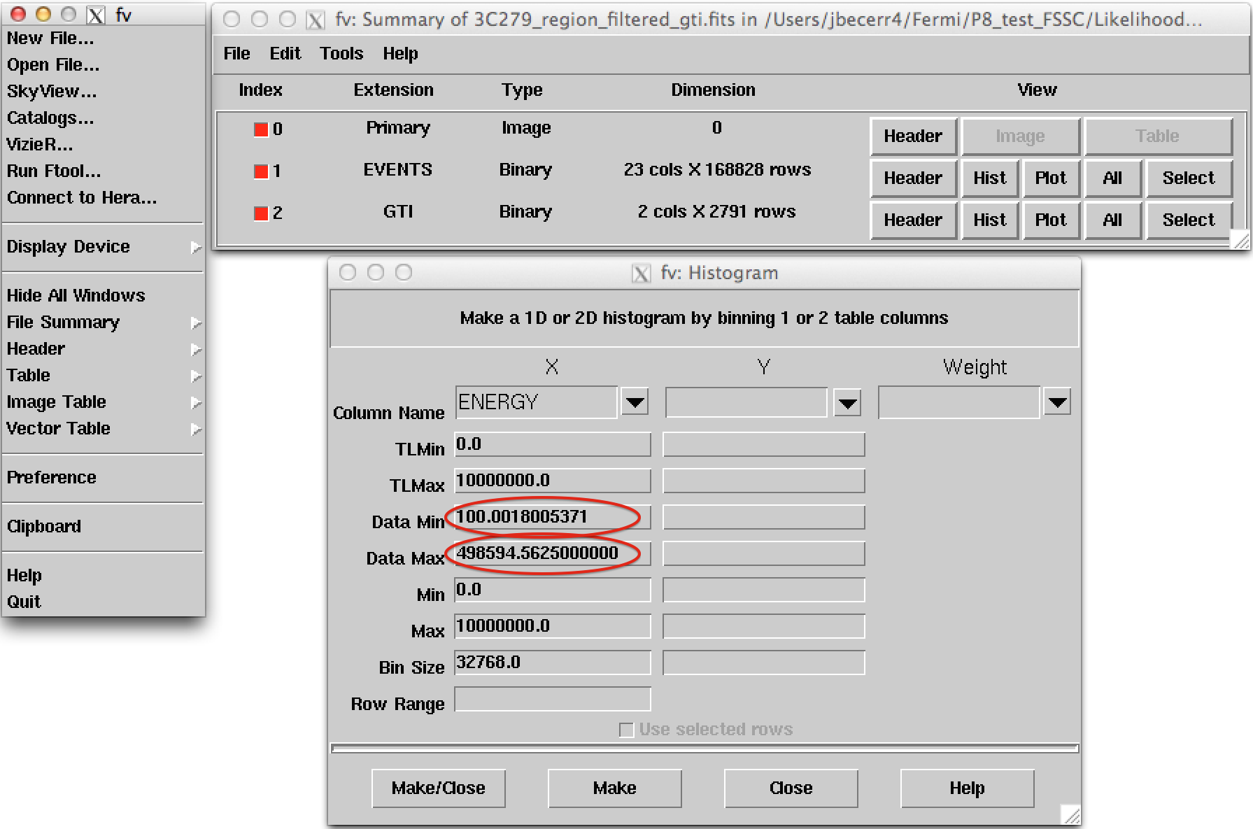
It is a good practice to check the maximum energy of the photons contained in our data sample. In this particular case, since we applied a maximum energy cut of 500 GeV, our statistics should be fine. However, if we try to go to higher energies, we might run out of photons and the likelihood fit will fail. To check the maximum energy, we can open the event file using e.g. fv:
!fv ./data/3C279_region_filtered_gti.fits
Click on the Hist button for the EVENTS extension. Then select for the X axis ENERGY.
The minimum and maximum energies are given by Data Min and Data Max. If Data Max is of the order of the maximum energy we used in our data selection we can proceed.
However, if Data Max is much smaller than the energy used in gtselect, then we need to come back to gtselect and make a tighter energy cut to make sure we will have enough statistics.
2. Make a counts map from the event data
Next, we create a counts map of the ROI, summed over photon energies, in order to identify candidate sources and to ensure that the field looks sensible as a simple sanity check. For creating the counts map, we will use the gtbin tool with the option CMAP as shown below:
%%bash
gtbin
    CMAP
    ./data/3C279_region_filtered_gti.fits
    ./data/3C279_region_filtered_gti_cmap.fits
    NONE
    160
    160
    0.25
    CEL
    193.98
    -5.82
    0.0
    AIT
NOTE: Here gtbin shows a warning due to the fact we are not using the spacecraft file. This is not a concern.
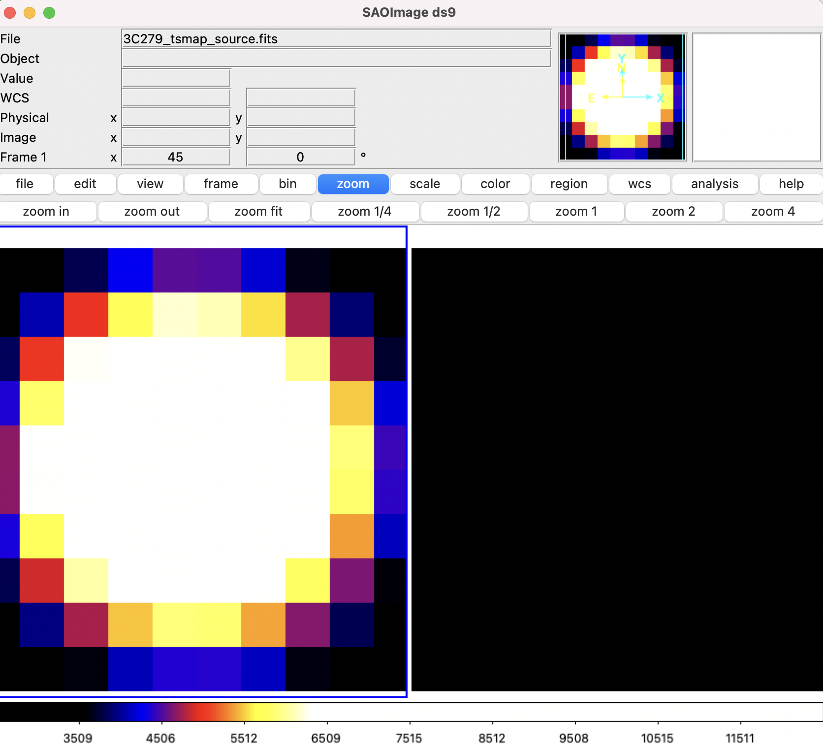
Now we can use the ds9 command to launch a visualization tool:
!ds9 ./data/3C279_region_filtered_gti_cmap.fits
ds9 produces this display:
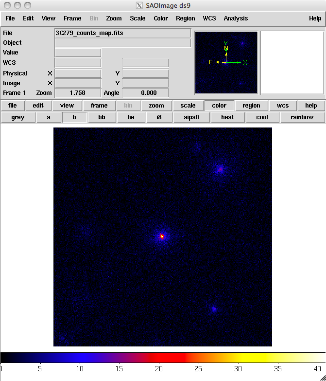
You can see one strong source and several weaker sources in this map. Mousing over the positions of these sources shows that two of them are likely 3C 279 and 3C 273.
It is important to inspect your data prior to proceeding to verify that the contents are as you expect. A malformed data query or improper data selection can generate a non-circular region, or a file with zero events.
By inspecting your data prior to analysis, you have an opportunity to detect such issues early in the analysis. (A more detailed discussion of data exploration can be found in the Explore LAT Data analysis thread.)
3. Make an exposure map
We are now ready to create an exposure map. The type of exposure map used by Likelihood differs significantly from the usual notion of exposure maps, which are essentially integrals of effective area over time. The exposure calculation that Likelihood uses consists of an integral of the total response over the entire ROI. See more information in the Cicerone.
Since the exposure calculation involves an integral over the ROI, separate exposure maps must be made for every distinct set of DSS cuts. This is important if, for example, one wants to subdivide an observation to look for secular flux variations from a particular source or sources. To view the DSS keywords in a given extension of a data file, use the gtvcut tool and review the data cuts for the EVENTS extension.
a. Generate a livetime cube
There are two tools needed for generating exposure maps. The first is gtltcube. This tool creates a livetimecube, which is a HealPix table, covering the full sky, of the integrated livetime as a function of inclination with respect to the LAT z-axis.
For more information about the livetime cubes, see the documentation in the Cicerone.
Here is the example of how to run gtltcube (this step takes several minutes):
%%bash
gtltcube zmax=90
    ./data/3C279_region_filtered_gti.fits
    ./data/spacecraft.fits
    ./data/3C279_ltcube.fits
    0.025
    1
NOTE: Values such as 0.1 for
Step size in cos(theta)are known to give unexpected reuslts. Use0.09instead.
The livetime cube generated for this analysis can be found here.
Since gtltcube produces a FITS file covering the entire sky, the output of this tool could be used for generating exposure maps for ROIs in other parts of the sky that have the same time interval selections.
But use caution! The livetime cube MUST be regenerated if you change any part of the time interval selection. This can occur by changing the start or stop time of the events, or simply by changing the energy selection or zenith angle cut (as these produce a different set of GTIs from gtmktime).
See e.g. Data Preparation in the Cicerone or the Data Preparation analysis thread.
Although the gtexpmap application (see below) can generate exposure maps for Likelihood without a livetime file, using one affords a substantial time savings.
b. Generate an exposure map.
The tool gtexpmap creates an exposure map based on the event selection used on the input photon file and the livetime cube. The exposure map must be recalculated if the ROI, zenith, energy selection or the time interval selection of the events is changed. For more information about the exposure maps see the documentation in the Cicerone.
Creating the exposure map using the gtexpmap tool, we have (this step can also take several minutes):
%%bash
gtexpmap
    ./data/3C279_region_filtered_gti.fits
    ./data/spacecraft.fits
    ./data/3C279_ltcube.fits
    ./data/3C279_unbin_expmap.fits
    CALDB
    30
    120
    120
    20
Note: If trying to use
CALDBin the example above does not work, just put the IRF name in explicitly. The appropriate IRF for this data set isP8R3_SOURCE_V3.
Note that we have chosen a 30 degree radius 'source region', while the acceptance cone radius specified for gtselect was 20 degrees. See the discussion of region selection in the Cicerone. This is necessary to ensure that events from sources outside the ROI are accounted for owing to the size of the instrument point-spread function (PSF).
Half-degree pixels are a nominal choice; smaller pixels should result in a more accurate evaluation of the diffuse source fluxes, but will also make the exposure map calculation itself lengthier.
The number of energies specifies the number of logarithmically spaced intervals bounded by the energy range given in the DSS keywords. A general recommendation is 10 bins per decade. This is sufficient to accommodate the change in effective area with energy near 100 MeV.
Here is one image plane of the exposure map we just created:
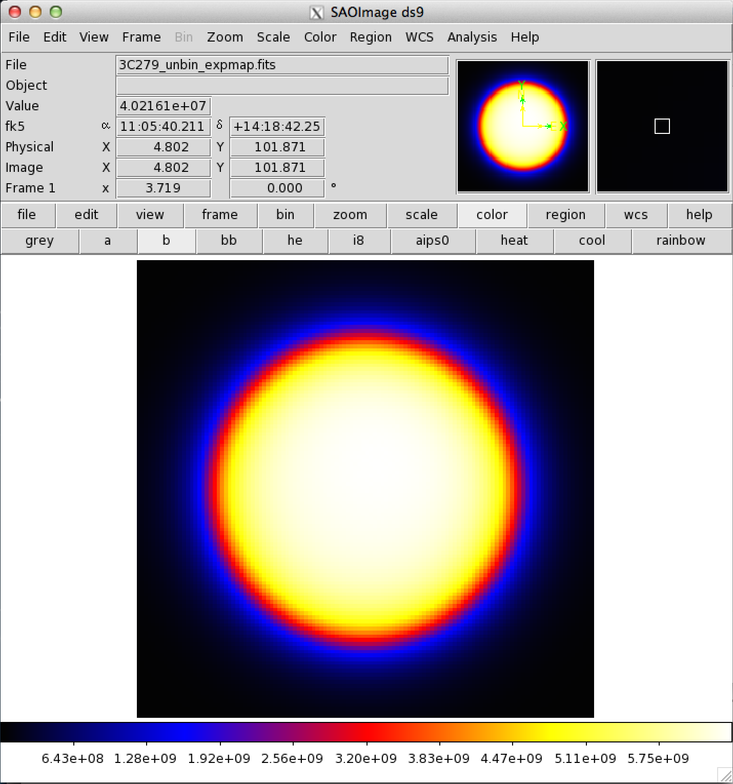
REMEMBER: The exposure needs to be recalculated if the ROI, zenith angle, time, event class, or energy selections applied to the data are changed.
4. Download the latest background models
When you use the current Galactic diffuse emission model (gll_iem_v07.fits) in a likelihood analysis, you also want to use the corresponding model for the extragalactic isotropic diffuse emission, which includes the residual cosmic-ray background. The recommended isotropic model for point source analysis is iso_P8R3_SOURCE_V3_v1.txt.
All the Pass 8 background models have been included in the Fermitools distribution in the $(FERMI_DIR)/refdata/fermi/galdiffuse/ directory. If you use that path in your model, you should not have to download the diffuse models individually.
NOTE: Keep in mind that the isotropic model needs to agree with both the event class and event type selections you are using in your analysis. The iso_P8R3_SOURCE_V3_v1.txt isotropic spectrum is valid only for the latest response functions and only for data sets with front + back events combined. All of the most up-to-date background models along with a description of the models are available here.
The gtlike tool reads the source model from an XML file. The model file contains your best guess at the locations and spectral forms for the sources in your data. A source model can be created using the model editor tool, by using the user contributed package LATSourceModel, or by editing the file directly within a text editor.
The example below illustrates how to install the LATSourceModel package. Note that this only needs to be done once after you have installed the Fermitools and activted that environment.
$ ln -s $FERMI_DIR/refdata/fermi/galdiffuse/gll_iem_v07.fits
$ ln -s $FERMI_DIR/refdata/fermi/galdiffuse/iso_P8R3_SOURCE_V3_v1.txt
(The model file you're about to download needs these files or symlinks to them in this directory)
Given the dearth of bright sources in the extraction region we have selected, our source model file will be fairly simple, comprising only the Galactic and Extragalactic diffuse emission, and point sources to represent the blazars 3C 279 and 3C 273. Here is an example XML file:
<?xml version="1.0" ?>
<source_library title="source library">

<!-- Point Sources -->

<source name="3C 273" type="PointSource">
<spectrum type="PowerLaw">
<parameter free="1" max="1000.0" min="0.001" name="Prefactor" scale="1e-09" value="10"/>
<parameter free="1" max="-1.0" min="-5.0" name="Index" scale="1.0" value="-2.1"/>
<parameter free="0" max="2000.0" min="30.0" name="Scale" scale="1.0" value="100.0"/>
</spectrum>
<spatialModel type="SkyDirFunction">
<parameter free="0" max="360" min="-360" name="RA" scale="1.0" value="187.25"/>
<parameter free="0" max="90" min="-90" name="DEC" scale="1.0" value="2.17"/>
</spatialModel>
</source>

<source name="3C 279" type="PointSource">
<spectrum type="PowerLaw">
<parameter free="1" max="1000.0" min="0.001" name="Prefactor" scale="1e-09" value="10"/>
<parameter free="1" max="-1.0" min="-5.0" name="Index" scale="1.0" value="-2"/>
<parameter free="0" max="2000.0" min="30.0" name="Scale" scale="1.0" value="100.0"/>
</spectrum>
<spatialModel type="SkyDirFunction">
<parameter free="0" max="360" min="-360" name="RA" scale="1.0" value="193.98"/>
<parameter free="0" max="90" min="-90" name="DEC" scale="1.0" value="-5.82"/>
</spatialModel>
</source>

<!-- Diffuse Sources -->
<source name="gll_iem_v07" type="DiffuseSource">
<spectrum type="PowerLaw">
<parameter free="1" max="10" min="0" name="Prefactor" scale="1" value="1"/>
<parameter free="0" max="1" min="-1" name="Index" scale="1.0" value="0"/>
<parameter free="0" max="2e2" min="5e1" name="Scale" scale="1.0" value="1e2"/>
</spectrum>
<spatialModel file="./gll_iem_v07.fits" type="MapCubeFunction">
<parameter free="0" max="1e3" min="1e-3" name="Normalization" scale="1.0" value="1.0"/>
</spatialModel>
</source>
<source name="iso_P8R3_SOURCE_V3_v1" type="DiffuseSource">
<spectrum file="./iso_P8R3_SOURCE_V3_v1.txt" type="FileFunction" apply_edisp="false">
<parameter free="1" max="10" min="1e-2" name="Normalization" scale="1" value="1"/>
</spectrum>
<spatialModel type="ConstantValue">
<parameter free="0" max="10.0" min="0.0" name="Value" scale="1.0" value="1.0"/>
</spatialModel>
</source>
</source_library>
The XML file used for this example is 3C279input_model.xml (in the cell below). For more details on the available XML models, see:
- Descriptions of available Spectral and Spatial Models
- Examples of XML Model Definitions for Likelihood
!wget https://fermi.gsfc.nasa.gov/ssc/data/analysis/scitools/data/Likelihood/3C279input_model.xml
!mv 3C279input_model.xml ./data
XML for Extended Sources
If your region includes any extended sources, you will need to add one or more extended sources to your XML model.
Download the extended source templates from the LAT Catalog page (look for "Extended Source template archive"). Extract the archive in the directory of your choice and note the path to the template files, which have names like W44.fits and VelaX.fits. You will need to modify your XML model so that the path to the template file is correct.
In addition, you will need to add the modifier map_based_integral='true' to the <spatialModel> atttribute. This modifier tells gtlike to use the proper integration method when evaluating the extended source.
Here is an example of the proper format for an extended source XML entry for Unbinned Likelihood analysis:
<?xml version="1.0" standalone="no"?>
<source_library title="source library">

<source name="W44" type="DiffuseSource">
<spectrum type="LogParabola" normPar="norm">
<parameter free="1" max="100000" min="1e-05" name="norm" scale="1e-11" value="2.891247798"/>
<parameter free="1" max="5" min="0" name="alpha" scale="1" value="2.399924084"/>
<parameter free="1" max="5" min="-1" name="beta" scale="1" value="0.2532196784"/>
<parameter free="0" max="300000" min="20" name="Eb" scale="1" value="1737.352167"/>
</spectrum>
<spatialModel file="./W44.fits" map_based_integral="true" type="SpatialMap">
<parameter free="0" max="1000" min="0.001" name="Prefactor" scale="1" value="1"/>
</spatialModel>
</source>

</source_library>
6. Compute the diffuse source responses
The diffuse source responses are computed by the gtdiffrsp tool.
The source model XML file must contain all of the diffuse sources to be fit. gtdiffrsp will add one column to the event data file for each diffuse source. The diffuse response depends on the instrument response function (IRF), which must be in agreement with the selection of events, i.e. the event class and event type we are using in our analysis. In this case we are using the standard SOURCE class (evclass=128) and event type 3 (FRONT+BACK), so we should use the IRF P8R3_SOURCE_V3 (which is the most commonly used in standard analysis).
Alternatively, you can just use CALDB for the IRF and the appropriate IRF will be automatically applied according to the previous event selection you performed during the previous steps of the analysis.
If the diffuse responses are not precomputed using gtdiffrsp, then the gtlike tool will compute them at runtime (during the next step). However, as this step is very computationally intensive (often taking ~hours to complete), and it is very likely you will need to run gtlike more than once, it is probably wise to precompute these quantities.
Here is an example of running gtdiffrsp:
%%bash
gtdiffrsp
    ./data/3C279_region_filtered_gti.fits
    ./data/spacecraft.fits
    ./data/3C279input_model.xml
    CALDB
Note: If trying to use CALDB in the example above does not work, just put the IRF name in explicitly. The appropriate IRF for this data set is
P8R3_SOURCE_V3.
There are a number of IRFs distributed with the Fermitools. Some of these IRFs, like P8R3_SOURCE_V3::FRONT, are designed to address only a subset of the events in the dataset, and thus would require you to make additional cuts before they could be used.
Once you have run gtdiffrsp, you can find the current names of the diffuse response column using the FTOOLS with:
fkeyprint <event file name>.fits DIFRSP
For example:
%%bash
fkeyprint
    ./data/3C279_region_filtered_gti.fits
    DIFRSP
The first part tells you the IRF name and, after the double underscore, the name of the diffuse component associated with the response.
If you are using a different IRF or diffuse model, you MUST compute a custom diffuse response prior to continuing the analysis.
Now we are ready to perform a likelihood analysis. You can get the resulting file, including the diffuse responses, here.
7. Run gtlike
We are now ready to run the gtlike application.
You may need the results of the likelihood fit to be output in XML model form (e.g. to use in generating a test statistic map).
To obtain an XML model output in addition to the standard results files, use the sfile parameter on the command line (as shown below) to designate the output XML model filename.
%%bash
gtlike refit=yes plot=yes sfile=3C279output_model.xml
    UNBINNED
    ./data/spacecraft.fits
    ./data/3C279_region_filtered_gti.fits
    ./data/3C279_unbin_expmap.fits
    ./data/3C279_ltcube.fits
    ./data/3C279input_model.xml
    CALDB
    NEWMINUIT
Most of the entries prompted for are fairly obvious.
In addition to the various XML and FITS files, the user is prompted for a choice of IRFs, the type of statistic to use, the optimizer, and some output file names.
The statistics available are:
UNBINNED: This is a standard unbinned analysis, described in this tutorial, to be used for short timescale or low source count data. If this option is chosen then parameters for the spacecraft file, event file, and exposure file must be given.
BINNED: This analysis is used for long timescale or high-density data (such as in the Galactic plane) which can cause memory errors in the unbinned analysis. See an explanation in the Binned Likelihood Tutorial.
There are five optimizers from which to choose: DRMNGB, DRMNFB, NEWMINUIT, MINUIT and LBFGS.
Generally speaking, the faster way to find the parameter estimates is to use DRMNGB (or DRMNFB) to find initial values and then use MINUIT (or NEWMINUIT) to find more accurate results.
If you have trouble achieving convergence at first, you can loosen your tolerance by setting the hidden parameter ftol on the command line. (The default value for ftol is 0.01.)
The application proceeds by reading in the spacecraft and event data, and if necessary, computing event responses for each diffuse source. If you get an error similar to this:
Caught St11range_error at the top level: Requested energy, 911163,
lies outside the range of the input file, 34.171, 877938
This means that we are trying to do our analysis beyond the maximum energy covered by the data sample. We should have checked that it was not the case during the data selection (as recommended in step 1).
To solve this issue we need to apply a harder cut in our event selection, setting the maximum energy within the energy range of available photons in your data sample.
Fortunately, this new event selection will not affect the time calculation (previous steps do not need to be repeated).
Here is the output from our fit with gtlike:
Minuit did successfully converge.

(MUCH OUTPUT OMITTED.)

Computing TS values for each source (4 total)
....!

Photon fluxes are computed for the energy range 100 to 500000 MeV

3C 273:
Prefactor: 9.53263 +/- 0.262701
Index: -2.63212 +/- 0.0212044
Scale: 100
Npred: 6369.65
ROI distance: 10.4409
TS value: 7810.96
Flux: 5.85022e-07 +/- 1.14156e-08 photons/cm^2/s

3C 279:
Prefactor: 7.3524 +/- 0.189805
Index: -2.20869 +/- 0.0144918
Scale: 100
Npred: 7420.98
ROI distance: 0
TS value: 13068.8
Flux: 6.08821e-07 +/- 1.08338e-08 photons/cm^2/s

gll_iem_v07:
Prefactor: 1.20506 +/- 0.0160704
Index: 0
Scale: 100
Npred: 95322.2
Flux: 0.000627754 +/- 8.37036e-06 photons/cm^2/s

iso_P8R3_SOURCE_V3:
Normalization: 1.05663 +/- 0.0281431
Npred: 47447.5
Flux: 0.000129821 +/- 3.45716e-06 photons/cm^2/s

WARNING: Fit may be bad in range [100, 549.28] (MeV)
WARNING: Fit may be bad in range [213340, 326604] (MeV)

Total number of observed counts: 156560
Total number of model events: 156560

-log(Likelihood): 1670346.65

Writing fitted model to 3C279output_model.xml
Since we selected plot=yes in the command line, a plot of the fitted data appears. (Note: Certain configurations are not producing a plot after gtlike. The FSSC is working on this issue at the moment. Please click here to generate a plot within python.)
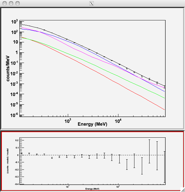
In the first plot, the counts/MeV vs MeV are plotted. The points are the data, and the lines are the models. Error bars on the points represent sqrt(Nobs) in that band, where Nobs is the observed number of counts. The black line is the sum of the models for all sources.
The colored lines follow the sources as follows:
- Black - summed model
- Red - first source in results.dat file (see below
- Green - second source
- Blue - third source
- Magenta - fourth source
In our case the 3C273 is the one in red, 3C279 is the one in green, the extragalactic background is blue, and the galactic background is magenta. If you have more sources, the colors are reused in the same order.
The second plot gives the residuals between your model and the data. Error bars here represent (sqrt(Nopbs))/Npred, where Npred is the predicted number of counts in each band based on the fitted model.
To assess the quality of the fit, look first for the words at the top of the output <Optimizer> did successfully converge. Successful convergence is a minimum requirement for a good fit.
Next, look at the energy ranges that are generating warnings of bad fits. If any of these ranges affect your source of interest, you may need to revise the source model and refit. You can also look at the residuals on the plot (bottom panel). If the residuals indicate a poor fit overall, you should consider changing your model file, perhaps by using a different source model definition and/or adding new sources in the ROI, and then refit the data.
If the fits and spectral shapes are good, but could be improved, you may wish to simply update your model file to hold some of the spectral parameters fixed.
For example, by fixing the spectral model for 3C 273, you may get a better quality fit for 3C 279. Close the plot and you will be asked if you wish to refit the data:
Refit? [y]n
Elapsed CPU time: 111.819315
prompt>
Here, hitting "return" will instruct the application to fit again. We are happy with the result, so we type n and end the fit.
Results
When it completes, gtlike generates a standard output XML file with the results of the fit.
If you re-run the tool in the same directory, these files will be overwritten by default. Use the clobber=no option on the command line to keep from overwriting the output files.
Unfortunately, the fit details and the value for the -log(likelihood) are not recorded in the automatic output files. You should consider logging the output to a text file for your records by using gtlike ... > fit_data.txt (or something similar) with your gtlike command.
Be aware, however, that this will make it impossible to request a refit when the likelihood process completes.
Example:
gtlike plot=no sfile=3C279output_model.xml > fit_data.txt
In this example, we used the sfile parameter to request that the model results be written to an output XML file, 3C279output_model.xml.
This file contains the source model results that were written to results.dat at the completion of the fit.
NOTE: If you have specified an output XML model file and you wish to modify your model while waiting at the
Refit? [y]prompt, you will need to copy the results of the output model file to your input model before making those modifications.
Errors reported with each value in the results.dat file are 1σ estimates (based on the inverse-Hessian at the optimum of the log-likelihood surface).
Other Useful Hidden Parameters
If you are scripting and wish to generate multiple output files without overwriting, the results and specfile parameters allow you to specify output filenames for the results.dat and counts_spectra.fits files respectively.
If you do not specify a source model output file with the sfile parameter, then the input model file will be overwritten with the latest fit. This is convenient as it allows the user to edit that file while the application is waiting at the Refit? [y] prompt so that parameters can be adjusted and set free or fixed. This would be similar to the use of the newpar, freeze, and thaw commands in XSPEC.
8. Make test-statistic maps
Ultimately, one would like to find sources near the detection limit of the instrument. To do this, you model the strongest, most obvious sources (with some theoretical prejudice as to the true source positions, e.g., assuming that most variable high Galactic latitude sources are blazars which can be localized by radio, optical, or X-ray observations), and then create "Test-statistic maps" to search for unmodeled point sources. These TS maps are created by moving a putative point source through a grid of locations on the sky and maximizing -log(likelihood) at each grid point, with the other, stronger, and presumably well-identified sources included in each fit. New, fainter sources are then identified at local maxima of the TS map.
The gttsmap tool can be run with or without an input source model. However, for a useful visualization of the results of the fit, it is recommended you use the output model file from gtlike. The file must be edited so all parameters are fixed (by setting the free attribute to 0 for each parameter) otherwise gttsmap will attempt a refit of the entire model at every point on the grid.
To see the field with the fitted sources removed (i.e. a residuals map), fix all point source parameters before running the TS map. See residuals map wget cell below.
To see the field with the fitted sources included, edit the model to remove all but the diffuse components. See sources map wget cell below.
# For residuals map: 3C279output_model_resid.xml
!wget https://fermi.gsfc.nasa.gov/ssc/data/analysis/scitools/data/Likelihood/3C279output_model_resid.xml
# For sources TS map: 3C279output_model_diffonly.xml
!wget https://fermi.gsfc.nasa.gov/ssc/data/analysis/scitools/data/Likelihood/3C279output_model_diffonly.xml
!mv *.xml ./data
In both cases, leave the Galactic diffuse prefactor (called Value in the model file) and the isotropic diffuse normalization parameters free during the fit.
Running gttsmap is extremely time-consuming, as the tool is performing a likelihood fit for all events at every pixel position. One way to reduce the time required for this step is to use very coarse binning and/or a very small region. In the following example, we run a TS map for the central 2.5x2.5 degree region of our data file, with .25 degree bins. This results in 100 maximum likelihood calculations. The run time for each of the maps discussed below was a few hours. A 20x20 degree region would require 6400 maximum likelihood calculations and will lengthen the run time significantly.
Here is an example of how to run the gttsmap tool to look for additional sources:
%%bash
gttsmap
    UNBINNED
    ./data/spacecraft.fits
    ./data/3C279_region_filtered_gti.fits
    ./data/3C279_unbin_expmap.fits
    ./data/3C279_ltcube.fits
    ./data/3C279output_model_resid.xml
    CALDB
    DRMNGB
    ./data/3C279_tsmap_resid.fits
    10
    10
    0.25
    CEL
    193.98
    -5.82
    AIT

#### Parameters
#### Takes a long time to run!
# Statistic to use (BINNED|UNBINNED)
# Spacecraft file
# Event file
# Unbinned exposure map
# Exposure hypercube file
# Source model file
# Response functions to use
# Optimizer (DRMNFB|NEWMINUIT|MINUIT|DRMNGB|LBFGS)
# TS map file name
# Number of X axis pixels
# Number of Y axis pixels
# Image scale (in degrees/pixel)
# Coordinate system (CEL|GAL)
# X-coordinate of image center in degrees (RA or l)
# Y-coordinate of image center in degrees (Dec or b)
# Projection method (AIT|ARC|CAR|GLS|MER|NCP|SIN|STG|TAN)
Note: If trying to use CALDB in the example above does not work, just put the IRF name in explicitly. The appropriate IRF for this data set is
P8R3_SOURCE_V3.
Because generating TS maps takes a long time, you may wish to download both the residuals and source files in the cells below.
# Residual file
!wget https://fermi.gsfc.nasa.gov/ssc/data/analysis/scitools/data/Likelihood/3C279_tsmap_resid.fits
# Source file
!wget https://fermi.gsfc.nasa.gov/ssc/data/analysis/scitools/data/Likelihood/3C279_tsmap_source.fits
!mv *.fits ./data
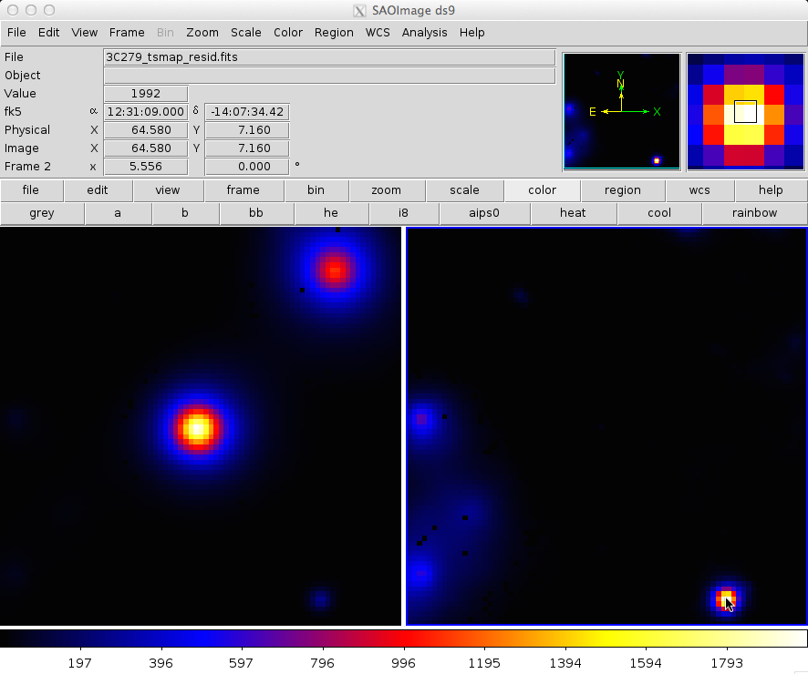
The output from the fit is below.
In the left panel, only diffuse sources were included in the analysis.
The right panel shows the same field, but with the point sources (3C 279 and 3C 273) included in the model, and thus not included in the output image.
This gives a pseudo-residuals map.
The location of the cursor in the image indicates the TS value at each position.
For comparison, we show a 20x20 degree of the same region that requires 6400 maximum likelihood calculations and takes a few days to complete. The bright source clearly seen in the lower part of this image is a recently identified millisecond pulsar.
NOTE: There may be a number of black pixels in these images where the likelihood fit did not converge. You should try adjusting the tolerance or using a different minimizer to keep this from happening.
In this example, the data set was small enough that an unbinned likelihood analysis is possible.
With longer data sets, however, you may run into memory allocation errors, at which time it is necessary to move to binned analysis for your region. A typical memory allocation error looks like:
gtlike(10869) malloc: *** mmap(size=2097152) failed (error code=12)*** error: can't allocate region*** set a breakpoint in malloc_error_break to debugIf you encounter this error, then Binned Likelihood analysis is for you!

- Curator: J.D. Myers
- NASA Official: Elizabeth Hays
- Fermi FAQ, Comments, Feedback
- › Privacy Policy and Important Notices
- › Accessibility
- › Contact NASA
- › Page Last Updated: Fri, Sep 15, 2023