
Please Note: An updated, and maintained, version of this content is available on the Livetime and Exposure page.
Livetime and Exposure
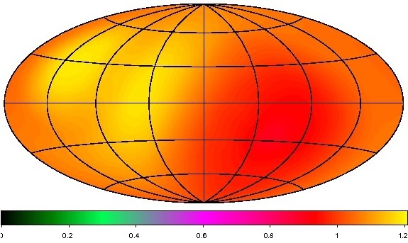
Here we want to create exposure maps for LAT data, to see the amount of time the LAT spent observing your region of interest.
Livetime Cube
The LAT instrument response functions are a function of the inclination angle, the angle between the direction to a source and the LAT normal. The number of counts that a source should produce should therefore depend on the amount of time that the source spent at a given inclination angle during an observation. This livetime quantity, the time that the LAT observed a given position on the sky at a given inclination angle, depends only on the history of the LAT's orientation during the observation and not on the source model. The array of these livetimes at all points on the sky is called the 'livetime cube.' As a practical matter, the livetime cubes are provided on a healpix grid on the sky and in inclination angle bins.
Livetime cubes are calculated by the gtltcube tool. The inputs are size of the spatial grid (in degrees), the inclination angle binning (in cos τ steps), and the spacecraft file (FT2). gtltcube calculates the livetime cube for the entire sky for the time range covered by the spacecraft file, and therefore the same output file can be used for analyzing different regions of the sky over the same time range.
Livetime cubes are additive: the livetime cube for a time range that is the sum of two time subranges is the sum of the livetime cube for each of the time subranges. Thus, the livetime cube for five calendar days can be calculated by adding the livetime cubes for each of the five calendar days. Livetime cubes can be added by gtltsum.
Exposure Maps
The type of exposure map used by Likelihood differs significantly from the usual notion of exposure maps, which are essentially integrals of effective area over time. The exposure calculation that Likelihood uses consists of an integral of the total response over the entire region-of-interest (ROI) data-space:
![]()
where primed quantities indicate measured energies, ![]() , and measured directions,
, and measured directions, ![]() . This exposure function can then be used to compute the
expected numbers of events from a given source:
. This exposure function can then be used to compute the
expected numbers of events from a given source:
![]()
where ![]() is the photon intensity from source
i. Since the exposure calculation involves an integral over
the ROI, separate exposure maps must be made for every distinct set of
DSS cuts if, for example, one wants to subdivide an observation to look
for secular flux variations from a particular source or sources.
is the photon intensity from source
i. Since the exposure calculation involves an integral over
the ROI, separate exposure maps must be made for every distinct set of
DSS cuts if, for example, one wants to subdivide an observation to look
for secular flux variations from a particular source or sources.
The exposure map is the total exposure—area multiplied by time—for a given position on the sky producing counts in your region of interest. Since the response function is a function of the photon energy, the exposure map is also a function of this energy. Thus the counts produced by a source at a given position on the sky is the integral of the source flux and the exposure map (a function of energy) at that position. The exposure map is used for extended sources such as the diffuse Galactic and Extragalactic backgrounds and not for individual sources.
The exposure map is calculated by the gtexpmap tool. The tool derives the Region of Interest from the observation's event file; remember that the region from which counts were selected is recorded by keywords in the photon file's FITS header. The Source Region is assumed to be centered on the Region of Interest, but the size of the Source Region must be input.
The gtexpmap tool needs the livetime spent at each inclination angle at every point in the Source Region; this can be provided by the livetime cube (as described in the previous subsection) or the tool will calculate these livetimes from the spacecraft file if no livetime cube file is provided. Note that the livetime cube is calculated on a spatial healpix grid while the exposure map is calculated on a longitude-latitude grid.
You control the rectilinear spatial grid: the number of pixels in each direction, their size, the coordinate system, the center of the grid, and the type of projection. Ten projections are provided (see Calabretta & Greisen 2002, A&A, 395, 1077); AIT for 'Aitoff' is suggested. You must also provide the instrument response function and the energy binning information: the energy range as well as the number of bins over which to perform the calculation. Binning is performed on a logarithmic energy scale.
gtexpcube makes the maps, printing out the energy and effective area for each map generated as it goes. Note: These maps are mono-energetic, and represent the exposure at the energy specified, not integrated over the band pass. The resulting exposure map files can then be viewed by fv or ds9. For examples, see the 'Explore the LAT data,' and 'Explore the LAT Data (Bursts)' threads. When you open the file, a "Data Cube" window will appear, allowing you to select between the various maps generated for each energy bin.
Combining Exposure
Generating each exposure map using gtexpcube is computationally intensive, as is combining these maps. Should you want to generate an exposure map covering multiple time intervals, it is recommended that you combine the livetime cubes using gtltsum prior to running gtexpcube, rather than combining the final exposure maps. gtltsum can only process a sum for two livetime cubes. So to sum more than two livetime cubes it will be necessary to run the gtltsum tool multiple times. Additionally, gtltsum will not allow you to overwrite an input file. Each filename must be unique.
» Forward to Likelihood Source Analysis
» Back to Counts Maps
» Back to the beginning of Data Exploration
» Back to the beginning of the Cicerone

- Curator: J.D. Myers
- NASA Official: Elizabeth Hays
- Fermi FAQ, Comments, Feedback
- › Privacy Policy and Important Notices
- › Accessibility
- › Contact NASA
- › Page Last Updated: Tue, Aug 05, 2025