Data

+ System Overview
+ Software Download
+ Documentation
+ Cicerone
+ Analysis Threads
+ User Contributions

LAT Gamma-Ray Burst Analysis

This procedure provides a step-by-step example of extracting and modeling a LAT Gamma-Ray Burst observation and modeling the prompt and temporally extended emissions using the X-Ray Spectral Fitting Package (Xspec) and gtlike, respectively. It should be noted that the LAT Low Energy (LLE) data products can also be used for LAT-detected GRBs (see GRB Analysis Using GTBurst).

You can download this tutorial as a Jupyter notebook and run it interactively. Please see the instructions for using the notebooks with the Fermitools.

Prerequisites

gtbin
gtdiffrsp
gtexpmap
gtfindsrc
gtltcube
gtmktime
gtrspgen
gtselect
gtvcut
XSPEC, used as a spectral analysis tool in Step 3 of this procedure (See Xanadu Data Analysis for X-Ray Astronomy.)
The FITS viewer fv
The astronomical imaging and data visualization application ds9

Assumptions

It is assumed that:

The referenced files reside in your working directory.
You know the time and location of the burst you wish to analyze.
Note: For this thread, we will analyze GRB080916C, one of the brightest LAT GRBs on record. The relevant burst properties are:
- T0 = 00:12:45.614 UT, 16 September 2008, corresponding to 243216766.614 seconds (MET)
- Trigger # 243216766
- RA = 121.8 degrees
- Dec = -61.3 degrees
You have extracted the files used in this tutorial; these files can be found here. Alternatively, you could download the LAT data for 080916C at the FSSC LAT Data server) using the above coordinates, a selection radius of 40 degrees, the energy range between 30 MeV and 300 GeV, and a time window in the range START=2008-09-16 00:04:26 (MET=243216266.6 s) and STOP=2008-09-16 00:46:05 (MET=243218766.6 s), corresponding to 500 and 2000 seconds before and after the trigger time, respectively. (The conversion between ISO 8601 date and MET can be performed using the HEASARC Time Conversion Utility). The instructions to generate the data and spacecraft files used in this section can be found in the Explore LAT Data (for Burst) analysis thread.
In this case, the GRB in question is of a sufficiently short duration, e.g. ~10's of seconds, so that the accumulation of LAT background counts is negligible. In order to study delayed emission, e.g. 10's of minutes to ~hour timescales, a likelihood analysis will be required.

Steps:

Localize the GRB.
Generating the analysis files.
Binned analysis with XSPEC (prompt emission).
Unbinned analysis using gtlike (extended emission).

NOTE: During the analysis of the prompt emission (Steps 1 to 3) we will make use of the P8R3_TRANSIENT020_V3 response function, while in the analysis of the extended emission (Step 4) the P8R3_SOURCE_V3 response function will be used.

1. Localize the GRB

a) Select LAT data during prompt burst phase

This can either be done using a time interval ascertained from data from other instruments (e.g., using the GBM trigger time and T90 values reported in the Fermi/GBM circular), or it can be estimated directly from the LAT light curve. Open the light curve "lc_zmax100.fits" (from the Explore LAT data thread or contained in the dowloaded tar file) with fv:


prompt> fv lc_zmax100.fits

LAT1_fvzmax100LCerrors

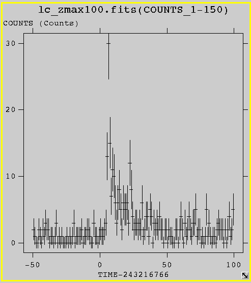
Here, we have plotted TIME-243216766 on the x-axis (with TIMEDEL as error) and COUNTS on the y-axis (with ERROR as error). Hovering the cursor over the plot will yield its x-y coordinates; in this case, a plausible estimate of the LAT emission interval is (T0, T0+40s).

We run gtselect to extract the data for this time interval. Remember to set "evclass=16" on the command line to ensure that we retain the transient class events:


  prompt> gtselect evclass=16

  Input FT1 file[] filtered_zmax100.fits

  Output FT1 file[] localize_zmax100.fits

  RA for new search center (degrees) (0:360) [INDEF]

  Dec for new search center (degrees) (-90:90) [INDEF]

  radius of new search region (degrees) (0:180) [INDEF] 15

  start time (MET in s) (0:) [INDEF] 243216766

  end time (MET in s) (0:) [INDEF] 243216806

  lower energy limit (MeV) (0:) [100]

  upper energy limit (MeV) (0:) [300000]

  maximum zenith angle value (degrees) (0:180) [180] 100

  Done.

Note that we have also reduced the acceptance cone to 15 degrees to filter out non-burst photons.

b) Run the localization tools, gtfindsrc and gtbin

If the data are essentially background-free as is the case here with a burst duration of ~50 sec, one can run the localization tools gtfindsrc and gtbin directly on the FT1 file (obtained when downloading the data file from the FSSC LAT Data server). gtfindsrc is necessary to centroid the GRB. For longer intervals where the background is significant, we can model the instrumental and celestial backgrounds using diffuse model components. For these data, the integration time is about 40 seconds so the diffuse and instrumental background components will make a negligible contribution to the total counts, so we proceed assuming they are negligible.

We run gtfindsrc first to find the local maximum of the log-likelihood of a point source model as well as an estimate of the error radius. We will use this information to specify the size of the TS map in order to ensure that it contains the error circles we desire.


prompt> gtfindsrc

Event file[localize_zmax100.fits] 

Spacecraft file[L1506171634094365357F22_SC00.fits] 

Output file for trial points[GRB080916C_gtfindsrc.txt] 

Response functions to use[P8_TRANSIENT020] P8R3_TRANSIENT020_V3

Livetime cube file[none] 

Unbinned exposure map[none] 

Source model file[none] 

Target source name[] 

Source '' not found in source model.

Enter coordinates for test source:

Coordinate system (CEL|GAL) [CEL] 

Intial source Right Ascension (deg) (-360:360) [0] 121.8

Initial source Declination (deg) (-90:90) [0] -61.3

Optimizer (DRMNFB|NEWMINUIT|MINUIT|DRMNGB|LBFGS) [MINUIT] 

Tolerance for -log(Likelihood) at each trial point[1e-2] 

Covergence tolerance for positional fit[0.01] 

Best fit position: 119.889,  -56.6719

Error circle radius: 0.0662923

In this example of running gtfindsrc the FT2.fits file was the renamed spacecraft data file downloaded from the FSSC LAT Data server. Since our source model comprises only a point source to represent the signal from the GRB, we do not provide a source model file or a target source name. Similarly, since the exposure map is used for diffuse components, we do not need to provide an unbinned exposure map. Use of a livetime cube will make the point source exposure calculation faster, but for integrations less than 1000 s, it is generally not needed.

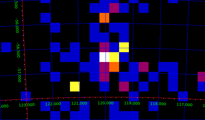
We have now obtained a position of maximum likelihood; we will use (119.861, -56.581) as our burst location from now on. It should be noted that GRB080916C is an exceptionally bright event in the LAT, and centroiding it with gtfindsrc is fast and adequate. In many other cases, a GRB may have far fewer LAT counts and the creation of a counts map using gtbin will be useful in localizing it:


prompt> gtbin

Type of output file (CCUBE|CMAP|LC|PHA1|PHA2) [] CMAP

Event data file name[] localize_zmax100.fits

Output file name[] GRB081916C_counts_map.fits

Spacecraft data file name[NONE] 

Size of the X axis in pixels[] 30

Size of the Y axis in pixels[] 30

Image scale (in degrees/pixel)[] 0.2

Coordinate system (CEL - celestial, GAL -galactic) (CEL|GAL) [] CEL

First coordinate of image center in degrees (RA or galactic l)[] 119.861

Second coordinate of image center in degrees (DEC or galactic b)[] -56.581

Rotation angle of image axis, in degrees[0.] 

Projection method e.g. AIT|ARC|CAR|GLS|MER|NCP|SIN|STG|TAN:[] AIT

gtbin: WARNING: No spacecraft file: EXPOSURE keyword will be set equal to ontime.

prompt>

We can now view the counts map in ds9:

LAT2_ds9tsmap

» Back to Top

2. Generating the analysis files

In this subsection, we'll use the same data we extracted as for the localization analysis above. The purpose is to illustrate the steps necessary to model a GRB that is significantly fainter than GRB080916C; i.e., one for which the residual and diffuse backgrounds need to be modeled. This means that we will include diffuse components in the model definition and that will necessitate the exposure map calculation in order for the code to compute the predicted number of events. We'll see from the fit to the data that these diffuse components do indeed provide a negligible contribution to the overall counts for this burst.

a) Data subselection

Rerun gtselect with (119.861, -56.581) as the new search center:


  prompt> gtselect evclass=16

  Input FT1 file[filtered_zmax100.fits]

  Output FT1 file[localize_zmax100.fits] prompt_select.fits

  RA for new search center (degrees) (0:360) [INDEF] 119.861

  Dec for new search center (degrees) (-90:90) [INDEF] -56.581

  radius of new search region (degrees) (0:180) [15]

  start time (MET in s) (0:) [243216766]

  end time (MET in s) (0:) [243216806]

  lower energy limit (MeV) (0:) [100]

  upper energy limit (MeV) (0:) [300000]

  maximum zenith angle value (degrees) (0:180) [100]

  Done.

b) Model definition

The model will include a point source at the GRB location, an isotropic component (to represent the extragalactic diffuse and/or the residual background), and a Galactic diffuse component that uses the recommend Galactic diffuse model, gal_2yearp7v6_v0.fits. This file is available at the LAT background models page via the FSSC Data Access page.

The easiest way to generate a simple 3 component model like this would be to use the modeleditor program (included in the Fermitools), by typing "modeleditor" at the prompt:

LAT3_modEd

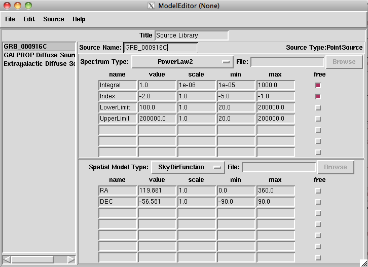
Here, we have added three sources to our model:

GRB_080916C (you can rename the source by typing into the "Source Name:" text input box), with a PowerLaw2 spectrum. (The Model Selection page of the Cicerone lists the possible spectral models.) We have adjusted the Lower Limit of its spectrum to be 100.0. We have also inputted the RA and Dec (calculated from gtfindsrc) into its spatial model. We have kept all other default values.
GALPROP Diffuse (there is a specific option for this in the "Source" menu). Edit the "File:" entry of the spatial model to point to your local copy of gll_iem_v07.fits. We have kept all other defaults.
Extragalactic Diffuse (there is a specific option for this). We have kept all the default values.

If our analysis region had been close to any known LAT sources, we would have had to include them in our model (see this tutorial).

The xml file GRB080916C_model.xml should look like this:


<?xml version="1.0" ?>

<source_library title="Source Library" xmlns="http://fermi.gsfc.nasa.gov/source_library">

  <source name="GRB_080916C" type="PointSource">

    <spectrum type="PowerLaw2">

      <parameter free="true" max="1000.0" min="1e-05" name="Integral" scale="1e-06" value="1.0"/>

      <parameter free="true" max="-1.0" min="-5.0" name="Index" scale="1.0" value="-2.0"/>

      <parameter free="false" max="200000.0" min="20.0" name="LowerLimit" scale="1.0" value="20.0"/>

      <parameter free="false" max="200000.0" min="20.0" name="UpperLimit" scale="1.0" value="200000.0"/>

    </spectrum>

    <spatialModel type="SkyDirFunction">

      <parameter free="false" max="360.0" min="0.0" name="RA" scale="1.0" value="119.861"/>

      <parameter free="false" max="90.0" min="-90.0" name="DEC" scale="1.0" value="-56.581"/>

    </spatialModel>

  </source>

  <source name="GALPROP Diffuse Source 1" type="DiffuseSource">

    <spectrum type="ConstantValue">

      <parameter free="true" max="10.0" min="0.0" name="Value" scale="1.0" value="1.0"/>

    </spectrum>

    <spatialModel file="$(FERMI_DIR)/refdata/fermi/galdiffuse/gll_iem_v07.fits" type="MapCubeFunction">

      <parameter free="false" max="1000.0" min="0.001" name="Normalization" scale="1.0" value="1.0"/>

    </spatialModel>

  </source>

  <source name="Extragalactic Diffuse Source 2" type="DiffuseSource">

    <spectrum type="PowerLaw">

      <parameter free="true" max="100.0" min="1e-05" name="Prefactor" scale="1e-07" value="1.6"/>

      <parameter free="false" max="-1.0" min="-3.5" name="Index" scale="1.0" value="-2.1"/>

      <parameter free="false" max="200.0" min="50.0" name="Scale" scale="1.0" value="100.0"/>

    </spectrum>

    <spatialModel type="ConstantValue">

      <parameter free="false" max="10.0" min="0.0" name="Value" scale="1.0" value="1.0"/>

    </spatialModel>

  </source>

</source_library>

You can also create and edit model files by hand rather than use the modeleditor, so long as the sources have the correct formats.

c) Refining the good time intervals (GTIs)

In general, our next step would be to run gtmktime to remove the time intervals whose events fell outside of our zenith angle cut and apply temporal cuts to the data based on the spacecraft file (FT2.fits). However, as our data encompasses a short period of time, this step is inappropriate in this case (gtmktime will report errors). It would be necessary if were analyzing a longer period of time such as a longer burst, or extended emission as at the end of this thread (see the Likelihood Tutorial for more information). Also, if we use gtvcut to review the file prompt_select.fits, we can see that the GTIs span the entire time selection we have made.

d) Diffuse response calculation

Since we are dealing with "evclass=16" (transient class) events, we need to run the gtdiffrsp tool. For each diffuse component in the model, the gtdiffrsp tool populates the "DIFRSP0" and "DIFRSP1" columns. They contain the integral over the source extent (for the Galactic and isotropic components this is essentially the entire sky) of the source intensity spatial distribution times the PSF and effective area. It computes the counts model density of the various diffuse components at each measured photon location, arrival time, and energy, and this information is used in maximizing the likelihood computation. This integral is also computed for the point sources in the model, but since those sources are delta-functions in sky position, the spatial part of the integral is trivial. Note that the large size of the new Galactic diffuse background model makes this a very resource-intensive process.


  prompt> gtdiffrsp

  Event data file[] prompt_select.fits

  Spacecraft data file[] FT2.fits

  Source model file[] GRB080916C_model.xml

  Response functions to use[P8R3_SOURCE_V3] P8R3_TRANSIENT020_V3

  adding source Extragalactic Diffuse Source 1

  adding source GALPROP Diffuse Source 0

  Working on...

  prompt_select.fits......................!

As mentioned before, gtdiffrsp modifies the input file by adding values to the "DIFRSP0" and "DIFRSP1" columns. In the tar file, for comparison purposes the user can find two copies of the input file, one used as input of gtdiffrsp (named "prompt_select_pre_gtdiffrsp.fits") and one obtained after running with gtdiffrsp and with the columns modified (named "prompt_select.fits").

e) Livetime cube generation

For analysis of longer time intervals, we would need to run gtltcube to calculate a livetime cube. For this analysis, this step is unnecessary due to the short timescales involved.

f) Exposure map generation

We now use gtexpmap to generate the exposure map. Note that the exposure maps from this tool are intended for use with unbinned likelihood analysis only:


  prompt> gtexpmap

  The exposure maps generated by this tool are meant

  to be used for *unbinned* likelihood analysis only.

  Do not use them for binned analyses.

  Event data file[] prompt_select.fits

  Spacecraft data file[] FT2.fits

  Exposure hypercube file[] none

  output file name[] prompt_expmap.fits

  Response functions[P8R3_SOURCE_V3] P8R3_TRANSIENT020_V3

  Radius of the source region (in degrees)[30] 25

  Number of longitude points (2:1000) [120] 100

  Number of latitude points (2:1000) [120] 100

  Number of energies (2:100) [20]

  Computing the ExposureMap (no expCube file given)

  ....................!

The radius of the source region should be larger than the extraction region in the FT1 data in order to account for PSF tail contributions of sources just outside the extraction region. For energies down to 100 MeV, a 10 degree buffer is recommended (i.e., the total radius is the sum of the extraction radius and the buffer area, totaling 25 in our case); for higher energy lower bounds, e.g., 1 GeV, 5 degrees or less is acceptable.

Again, note that we did not provide an "exposure hypercube" (the livetime cube) file. For data durations less than about 1ks, gtexpmap will execute faster doing the time integration over the livetimes in the FT2 file directly. For longer integrations, computing the livetime cube with gtltcube will be faster (more information can be found in the Explore LAT Data section). At this step, the flux and spectral shape of the GRB prompt emission can be estimated using the gtlike tool (see section 4f).

» Back to Top

3. Binned analysis with XSPEC (prompt emission)

We will now perform a spectral analysis on the prompt emission using XSPEC. (A basic knowledge of the use of XSPEC is assumed.) This requires a PHA (spectral) file and a RSP (response) file. It should be noted that as an alternative to XSPEC, the RMFIT software (available as a user contribution) can be used for spectral modeling; however, it is not distributed as part of the Fermitools.

a) Generating PHA and RSP files

We use gtbin to create the PHA1 file (the choice of PHA1 for 'Type of output file' indicates that you want to create a PHA file — the standard FITS file containing a single binned spectrum — spanning the entire time range):


  prompt> gtbin

  Type of output file (CCUBE|CMAP|LC|PHA1|PHA2) [LC] PHA1

  Event data file name[filtered_zmax100.fits] prompt_select.fits

  Output file name[lc_zmax100.fits] 080916C_LAT.pha

  Spacecraft data file name[FT2.fits]

  Algorithm for defining energy bins (FILE|LIN|LOG) [LOG]

  Start value for first energy bin in MeV[30] 100

  Stop value for last energy bin in MeV[200000] 300000

  Number of logarithmically uniform energy bins[20] 30

The gtrspgen tool is then run to generate an XSPEC-compatible response matrix from the LAT IRFs.


  prompt> gtrspgen

  Response calculation method (GRB|PS) [GRB] PS

  Spectrum file name[] 080916C_LAT.pha

  Spacecraft data file name[] FT2.fits

  Output file name[] 080916C_LAT.rsp

  Cutoff angle for binning SC pointings (degrees)[60.] 90

  Size of bins for binning SC pointings (cos(theta))[.05]

  Response function to use, CALDB or irf name [CALDB] CALDB

  Algorithm for defining true energy bins (FILE|LIN|LOG) [LOG]

  Start value for first energy bin in MeV[30.] 100

  Stop value for last energy bin in MeV[200000.] 300000

  Number of logarithmically uniform energy bins[100]

Notes:

One should always use the "PS" response calculation method, despite the option of using "GRB". The latter was a method used in the early stages of the software creation but was later never fully developed. Ultimately, the "PS" method should always be more accurate, in particular for longer bursts. For short bursts, the difference in results and execution time between "PS" and "GRB" is negligible.
In gtrspgen you choose the incident photon energy bins; i.e., the energy bins over which the incident photon model is computed. gtrspgen reads the output photon channel energy grid from the PHA file. The RSP created by gtrspgen is the mapping from the incident photon energy bins into the output photon channels. These incident photon energy bins need not be the same as the output channels and they should generally over-sample them:
- If there are only a few channels then the calculation of the expected number of photons in each channel will be more accurate if there are more incident photon energy bins.
- You might want to include some incident photon energy bins above and below the range of channels to account for the LAT's finite energy resolution. Incident energy bins above the highest channel energy is particularly important if some for the photon's energy leaks out of the detector.

b) Backgrounds

For the prompt emission of GRB 080916C (and most LAT bursts), there is minimal background contamination. For analyses of longer integrations, one can estimate the background using off-source regions as for more traditional X-ray analyses.

c) Running XSPEC

You now have the two files necessary to analyze the burst spectrum with XSPEC:

A PHA file with the spectrum.
A RSP file with the response function.

Note that there is no background file. All non-burst sources are expected to produce less than 1 photon in the extraction region during the burst! Here we provide the simplest example of fitting a spectrum with XSPEC; for further details you should consult the XSPEC manual.

1. Start XSPEC

Note: The default version is now release 12 (XSPEC12).

2. Load in the data:


    XSPEC12> data 080916C_LAT.pha

    ***Warning: No TLMIN keyword value for response matrix FCHAN column.

                    Will assume TLMIN = 1.

    

    1 spectrum  in use

    

    Spectral Data File: 080916C_LAT.pha  Spectrum 1

    Net count rate (cts/s) for Spectrum:1  4.919e+00 +/- 3.815e-01

    Assigned to Data Group 1 and Plot Group 1

    Noticed Channels:  1-30

    Telescope: GLAST Instrument: LAT  Channel Type: PI

    Exposure Time: 37 sec

    Using fit statistic: chi

    Using Response (RMF) File        080916C_LAT.rsp for Source 1

When you specify a data file, XSPEC will try to load the response file in the PHA file's header. Alternatively, you can specify the response file separately with the command "response 080916C_LAT.rsp".

We now load in a power law model for fitting the data. For more information on available models, see this example.

3. Load the model:


    XSPEC12> model pow

    

    Input parameter value, delta, min, bot, top, and max values for ...

                  1       0.01         -3         -2          9         10

    1:powerlaw:PhoIndex>

                  1       0.01          0          0      1e+24      1e+24

    2:powerlaw:norm>

    

    ========================================================================

        Model powerlaw<1> Source No.: 1   Active/On

        Model Model Component  Parameter  Unit     Value

         par  comp

           1    1   powerlaw   PhoIndex            1.00000      +/-  0.0

           2    1   powerlaw   norm                1.00000      +/-  0.0

    ________________________________________________________________________

     

     Chi-Squared =   8.440734e+10 using 30 PHA bins.

     Reduced chi-squared =   3.014548e+09 for     28 degrees of freedom

     Null hypothesis probability =   0.000000e+00

     Current data and model not fit yet.

4. Set XSPEC to plot the data and to select the statistical methood for fitting:


    XSPEC12> cpd /xs

    XSPEC12> setplot energy 

    XSPEC12> plot ldata chi

    ***Warning: Fit is not current.

    XSPEC12> statistic cstat

    Warning: Cstat statistic is only valid for Poisson data.

    cstat statistic: variance weighted using standard weighting

    

    C-statistic =   3.369254e+06 using 30 PHA bins and 28 degrees of freedom.

    

    Warning: Cstat statistic is only valid for Poisson data.

    

    Current data and model not fit yet.

The "cpd" command sets the current plotting device, which in this case is the "xserve" option (an xwindow that persists after XSPEC has been closed). The next two commands tell XSPEC to create a logarithmic (the "l" of "ldata") plot of the energy (along the x-axis), using the data file specified before, with the fit statistic. (Consult the manual for another example.)

It is important to note that, for LAT GRB analysis, we generally want to use the C-statistic instead of chi-squared due to the small number of counts. (However, the command for plotting is still "chi" or "chisq" regardless of the statistic used.) We have set this in the last step.

5. Perform a fit, and plot the results:


XSPEC12> fit



<...skip output...>



========================================================================

Model powerlaw<1> Source No.: 1   Active/On

Model Model Component  Parameter  Unit     Value

 par  comp

   1    1   powerlaw   PhoIndex            2.30022      +/-  7.70503E-02

   2    1   powerlaw   norm                5715.50      +/-  5583.06

________________________________________________________________________

    

    C-statistic =          26.57 using 30 PHA bins and 28 degrees of freedom.

    

    Warning: Cstat statistic is only valid for Poisson data.

    Source file is not Poisson

    

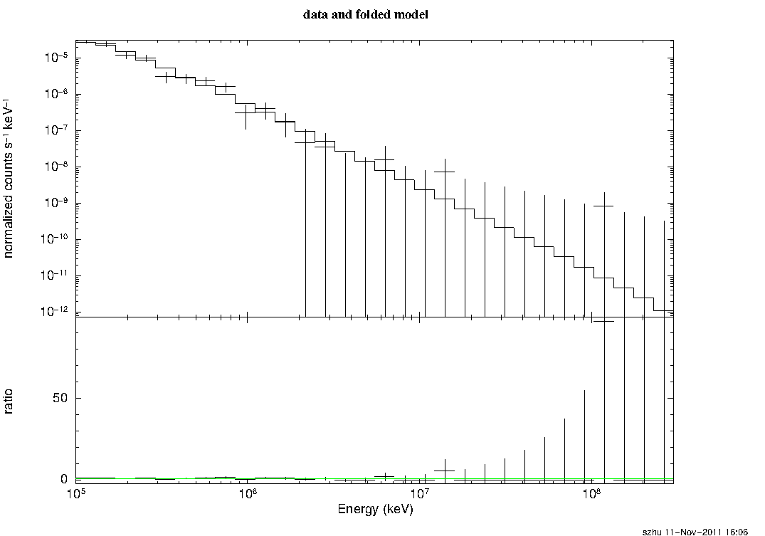
XSPEC12> plot ldata resid

LAT4_xspec_ldata_res


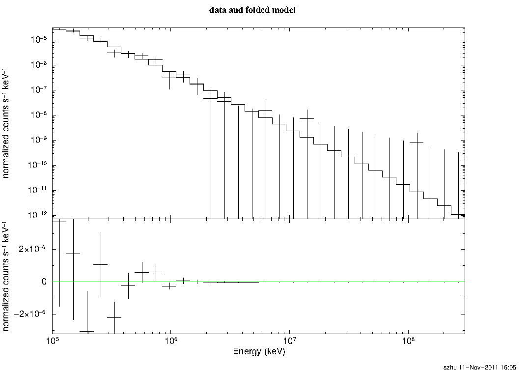
XSPEC12> plot ldata ratio

LAT5_xspec_ldata_ratio

» Back to Top

4. Unbinned analysis using gtlike (temporally extended emission)

a) Data subselection

Here, we will search for emission which may occur after the prompt GRB event; temporally extended high-energy emission has been detected in a large number of LAT bursts. We rerun gtselect on a time interval of ~40 to 400 seconds after the trigger on the file downloaded from the archive and renamed "FT1.fits", choosing to exclude "transient" class photons for the analysis of extended emission. (A longer interval has been chosen to demonstrate gtmktime, gtltcube, etc.) Remember to set "evclass=128" on the command line to ensure that we use the source class events.


  promp> gtselect evclass=128

  Input FT1 file[filtered_zmax100.fits] FT1.fits

  Output FT1 file[prompt_select.fits] extended_select.fits

  RA for new search center (degrees) (0:360) [119.861]

  Dec for new search center (degrees) (-90:90) [-56.581]

  radius of new search region (degrees) (0:180) [15]

  start time (MET in s) (0:) [243216766] 243216806

  end time (MET in s) (0:) [243216806] 243217166

  lower energy limit (MeV) (0:) [100]

  upper energy limit (MeV) (0:) [300000]

  maximum zenith angle value (degrees) (0:180) [100]

  Done.

b) Refining the GTIs

Since our subselection encompasses a longer period of time, we run gtmktime to exclude bad time intervals with the filter expression suggested in the Cicerone:


  prompt> gtmktime

  Spacecraft data file[] FT2.fits

  Filter expression[(DATA_QUAL>0)&&(LAT_CONFIG==1)]

  Apply ROI-based zenith angle cut[yes]

  Event data file[] extended_select.fits

  Output event file name[] extended_mktime.fits

Note: In an analysis of transient class events, we set the data quality portion of the filter expression to "DATA_QUAL>0" to retain these events.

c) Diffuse response calculation

We run now gtdiffrsp, making sure to use the correct response function. Again, note that the pass 8 Galactic diffuse background model causes this to be very resource-intensive. The tool modifies the input event data file, inserting values in the "DIFRSP0" and "DIFRSP1" columns. A copy of the input file (named "extended_mktime_pre_gtdiffrsp.fits"), generated before running gtdiffrsp, can be found in the tar file.


  prompt> gtdiffrsp

  Event data file[prompt_select.fits] extended_mktime.fits

  Spacecraft data file[] FT2.fits

  Source model file[] GRB080916C_model.xml

  Response functions to use[P8R3_TRANSIENT020_V3] P8R3_SOURCE_V3

  adding source Extragalactic Diffuse Source 1

  adding source GALPROP Diffuse Source 0

  Working on...

  extended_mktime.fits..............................!

d) Livetime cube generation

Now that our data file encompasses a longer period of time, it requires us to calculate the livetime cube using gtltcube:


  prompt> gtltcube

  Event data file[] extended_mktime.fits

  Spacecraft data file[] FT2.fits

  Output file[expCube.fits] extended_ltcube.fits

  Step size in cos(theta) (0.:1.) [0.025]

  Pixel size (degrees)[1] 0.5

  Working on file FT2.fits

  ............!

e) Exposure map generation

This time we will specify a livetime cube file:


  prompt> gtexpmap

  The exposure maps generated by this tool are meant

  to be used for *unbinned* likelihood analysis only.

  Do not use them for binned analyses.

  Event data file[prompt_select.fits] extended_mktime.fits

  Spacecraft data file[] FT2.fits

  Exposure hypercube file[none] extended_ltcube.fits

  output file name[prompt_expmap.fits] extended_expmap.fits

  Response functions[P8R3_TRANSIENT020_V3] P8R3_SOURCE_V3

  Radius of the source region (in degrees)[25]

  Number of longitude points (2:1000) [100]

  Number of latitude points (2:100) [100]

  Number of energies (2:100) [20]

  Computing the ExposureMap using extended_ltcube.fits

  ....................!

f) Calculating the likelihood

We will use gtlike for this analysis. The "plot=yes" command brings up a plot of the fit results; "results=results.dat" saves a copy of the fit results to the file "results.dat".


prompt> gtlike plot=yes results=results.dat

Statistic to use (BINNED|UNBINNED) [UNBINNED] 

Spacecraft file[none] FT2.fits

Event file[none] extended_mktime.fits

Unbinned exposure map[none] extended_expmap.fits

Exposure hypercube file[none] extended_ltcube.fits

Source model file[] GRB080916C_model.xml

Response functions to use[CALDB] P8R3_SOURCE_V3

Optimizer (DRMNFB|NEWMINUIT|MINUIT|DRMNGB|LBFGS) [MINUIT] 



<...skip output...>



Computing TS values for each source (3 total)

...!



Photon fluxes are computed for the energy range 100 to 300000 MeV



Extragalactic Diffuse Source 1:

Prefactor: 22.7243 +/- 7.97519

Index: -2.1

Scale: 100

Npred: 46.5995

Flux: 0.00259734 +/- 0.000910953 photons/cm^2/s



GALPROP Diffuse Source 0:

Value: 3.89072 +/- 1.22098

Npred: 52.397

Flux: 0.0019012 +/- 0.000596581 photons/cm^2/s



GRB_080916C:

Integral: 0.999997 +/- 31.6067

Index: -2 +/- 1.73205

LowerLimit: 20

UpperLimit: 200000

Npred: 2.60323e-09

ROI distance: 105.916

TS value: -1.33844e-07

Flux: 2.00062e-07 +/- 6.34438e-06 photons/cm^2/s



WARNING: Fit may be bad in range [740.083, 1104.43] (MeV)

WARNING: Fit may be bad in range [1648.13, 2459.51] (MeV)



Total number of observed counts: 99

Total number of model events: 98.9964



-log(Likelihood): 833.7808648

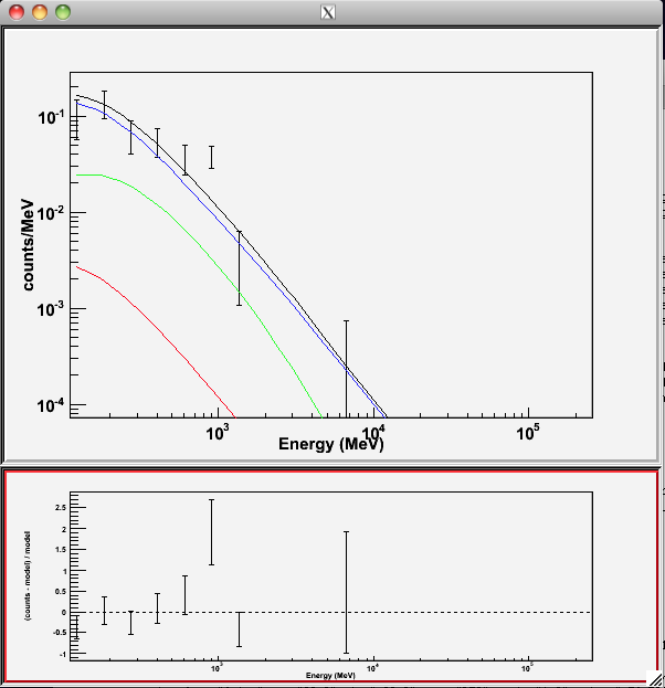
The plot produced by gtlike shows the fitting results: The red, green, and blue lines correspond to the fit of the extragalactic diffuse background, the galactic diffuse background, and the GRB, respectively (as explained in the Run gtlike section of the Likelihood Tutorial). The black line is the sum of the 3 components.

In our model, we included the galactic and extragalactic diffuse backgrounds. In a real analysis, we would have also included any known sources within ~20 or so degrees of the burst.

LAT6_gtlike

» Back to Top

Last updated by: N. Mirabal - 02/27/2018

National Aeronautics and Space Administration

Goddard Space Flight Center

Data

LAT Gamma-Ray Burst Analysis

Prerequisites

Assumptions

Steps:

1. Localize the GRB

2. Generating the analysis files

3. Binned analysis with XSPEC (prompt emission)

a) Generating PHA and RSP files

b) Backgrounds

c) Running XSPEC

1. Start XSPEC

2. Load in the data:

3. Load the model:

4. Set XSPEC to plot the data and to select the statistical methood for fitting:

5. Perform a fit, and plot the results:

4. Unbinned analysis using gtlike (temporally extended emission)